What-if Analysis
Introduction
Excel includes many powerful tools to perform complex mathematical calculations, including what-if analysis. This feature can help you experiment and answer questions with your data, even when the data is incomplete. In this lesson, you will learn how to use a what-if analysis tool called Goal Seek.
Optional: Download our practice workbook.
- Watch the video below to learn more about what-if analysis and Goal Seek.
Goal Seek
Whenever you create a formula or function in Excel, you put various parts together to calculate a result. Goal Seek works in the opposite way: It lets you start with the desired result, and it calculates the input value that will give you that result. We'll use a few examples to show how to use Goal Seek.
To use Goal Seek (example 1):
Let's say you're enrolled in a class. You currently have a grade of 65, and you need at least a 70 to pass the class. Luckily, you have one final assignment that might be able to raise your average. You can use Goal Seek to find out what grade you need on the final assignment to pass the class.
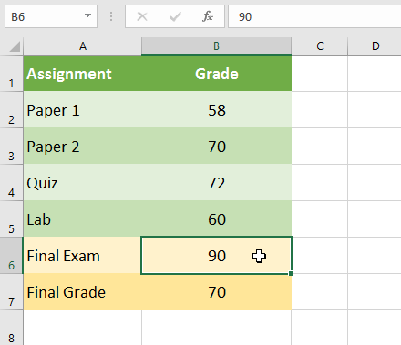
In the image below, you can see that the grades on the first four assignments are 58, 70, 72, and 60. Even though we don't know what the fifth grade will be, we can write a formula—or function—that calculates the final grade. In this case, each assignment is weighted equally, so all we have to do is average all five grades by typing =AVERAGE(B2:B6). Once we use Goal Seek, cell B6 will show us the minimum grade we'll need to make on that assignment.
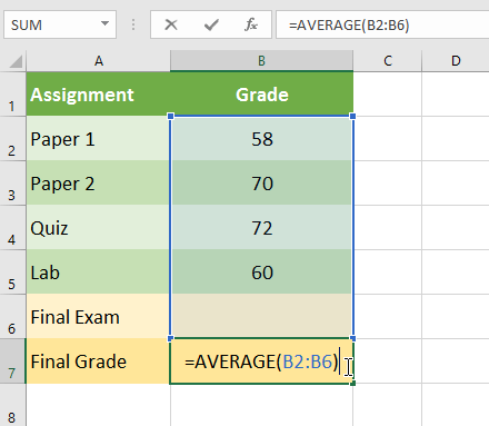
- Select the cell with the value you want to change. Whenever you use Goal Seek, you'll need to select a cell that already contains a formula or function. In our example, we'll select cell B7 because it contains the formula =AVERAGE(B2:B6).
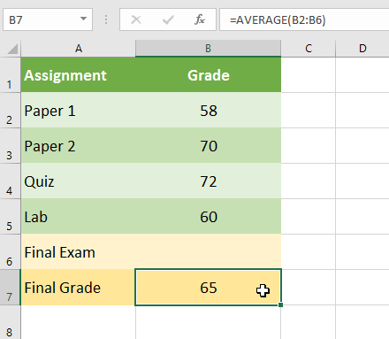
- From the Data tab, click the What-If Analysis command, then select Goal Seek from the drop-down menu.

- A dialog box will appear with three fields. The first field, Set cell:, will contain the desired result. In our example, cell B7 is already selected.
The second field, To value:, is the desired result. In our example, we'll enter 70 because we need to earn at least that to pass the class.
The third field, By changing cell:, is the cell where Goal Seek will place its answer. In our example, we'll select cell B6 because we want to determine the grade we need to earn on the final assignment. - When you're done, click OK.
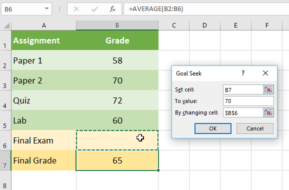
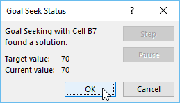
- The dialog box will tell you if Goal Seek was able to find a solution. Click OK.
- The result will appear in the specified cell. In our example, Goal Seek calculated that we will need to score at least a 90 on the final assignment to earn a passing grade.
To use Goal Seek (example 2):
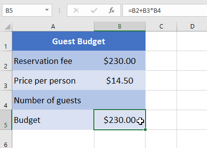
Let's say you're planning an event and want to invite as many people as you can without exceeding a budget of $500. We can use Goal Seek to figure out how many people to invite. In our example below, cell B5 contains the formula =B2+B3*B4 to calculate the total cost of a room reservation, plus the cost per person.
- Select the cell with the value you want to change. In our example, we'll select cell B5.
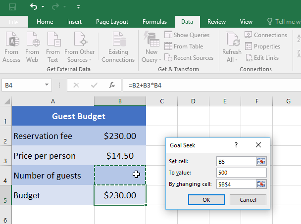
- From the Data tab, click the What-If Analysis command, then select Goal Seek from the drop-down menu.

- A dialog box will appear with three fields. The first field, Set cell:, will contain the desired result. In our example, cell B5 is already selected.
The second field, To value:, is the desired result. In our example, we'll enter 500 because we only want to spend $500.
The third field, By changing cell:, is the cell where Goal Seek will place its answer. In our example, we'll select cell B4 because we want to know how many guests we can invite without spending more than $500. - When you're done, click OK.
- The dialog box will tell you if Goal Seek was able to find a solution. Click OK.
- The result will appear in the specified cell. In our example, Goal Seek calculated the answer to be approximately 18.62. In this case, our final answer needs to be a whole number, so we'll need to round the answer up or down. Because rounding up would cause us to exceed our budget, we'll round down to 18 guests.
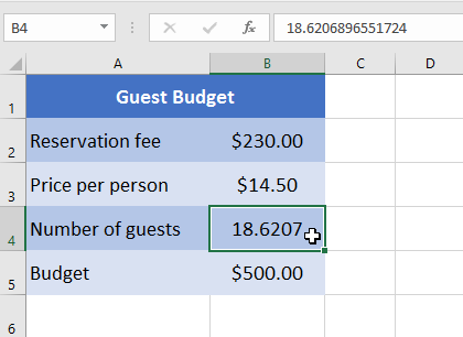
As you can see in the example above, some situations will require the answer to be a whole number. If Goal Seek gives you a decimal, you'll need to round up or down, depending on the situation.
Other types of what-if analysis
For more advanced projects, you may want to consider the other types of what-if analysis: scenarios and data tables. Instead of starting from the desired result and working backward, like with Goal Seek, these options allow you to test multiple values and see how the results change.
- Scenarios let you substitute values for multiple cells (up to 32) at the same time. You can create as many scenarios as you want and then compare them without changing the values manually. In the example below, we're using scenarios to compare different venues for an upcoming event.
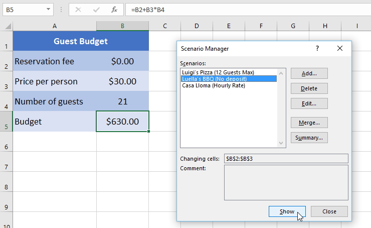
For more information on scenarios, check out this article from Microsoft.
- Data tables allow you to take one or two variables in a formula and replace them with as many different values as you want, then view the results in a table. This option is especially powerful because it shows multiple results at the same time, unlike scenarios or Goal Seek. In the example below, we can view 24 possible results for a car loan.
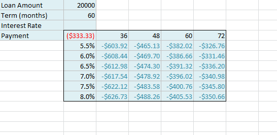
For more information on data tables, check out this article from Microsoft.
Challenge!
- Open our practice workbook.
- Click the Challenge tab in the bottom-left of the workbook.
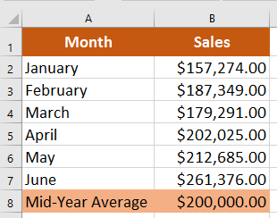
- In cell B8, create a function that calculates the average of the sales in B2:B7.
- The workbook shows Dave's monthly sales amounts for the first half of the year. If he reaches a $200,000 mid-year average, he will receive a 5% bonus. Use Goal Seek to find how much he needs to sell in June in order to make the $200,000 average.
- When you're finished, your workbook should look like this:
