Doing More with PivotTables
Introduction
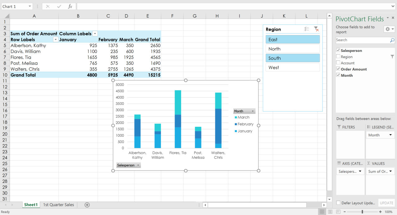
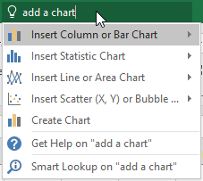
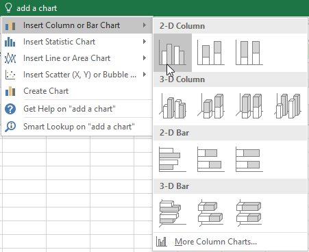
As you learned in our previous lesson, Intro to PivotTables, PivotTables can be used to summarize and analyze almost any type of data. To help you manipulate your PivotTable—and gain even more insight into your data—Excel offers three additional tools: filters, slicers, and PivotCharts.
Optional: Download our practice workbook.
- Watch the video below to learn more about enhancing PivotTables.
Introduction
Excel is a spreadsheet program that allows you to store, organize, and analyze information. While you may believe Excel is only used by certain people to process complicated data, anyone can learn how to take advantage of the program's powerful features. Whether you're keeping a budget, organizing a training log, or creating an invoice, Excel makes it easy to work with different types of data.
Watch the video below to learn more about Excel.
Getting to know Excel
If you've previously used Excel 2010 or Excel 2013, then Excel 2016 should feel familiar. If you are new to Excel or have more experience with older versions, you should first take some time to become familiar with the Excel interface.
The Excel interface
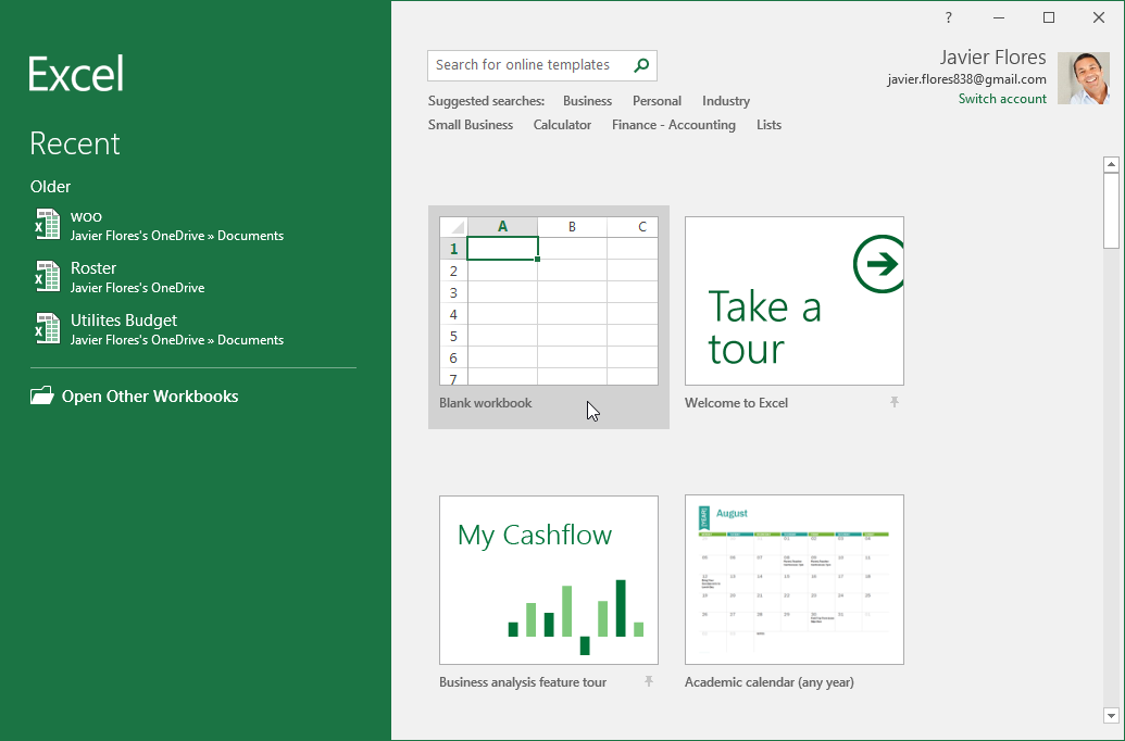
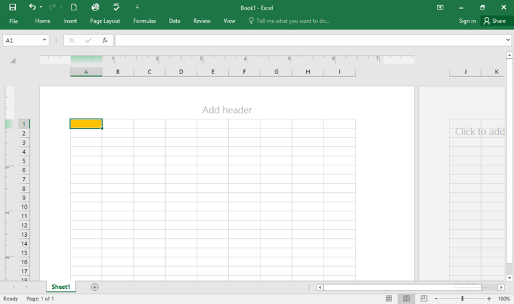
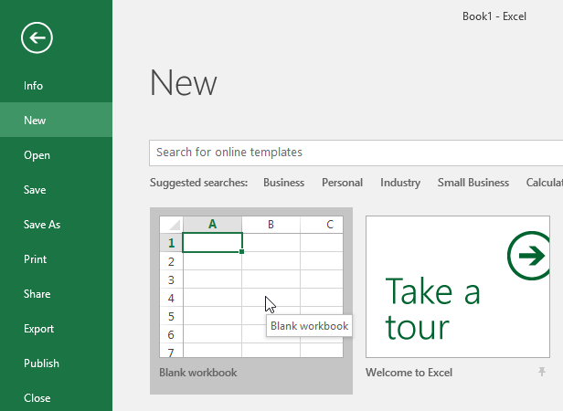
When you open Excel 2016 for the first time, the Excel Start Screen will appear. From here, you'll be able to create a new workbook, choose a template, and access your recently edited workbooks.
- From the Excel Start Screen, locate and select Blank workbook to access the Excel interface.
Click the buttons in the elow to become familiar with the Excel interface.
Working with the Excel environment
The Ribbon and Quick Access Toolbar are where you will find the commands to perform common tasks in Excel. The Backstage view gives you various options for saving, opening a file, printing, and sharing your document.
The Ribbon
Excel 2016 uses a tabbed Ribbon system instead of traditional menus. The Ribbon contains multiple tabs, each with several groups of commands. You will use these tabs to perform the most common tasks in Excel.
- Each tab will have one or more groups.
- Some groups will have an arrow you can click for more options.
- Click a tab to see more commands.
- You can adjust how the Ribbon is displayed with the Ribbon Display Options.
Certain programs, such as Adobe Acrobat Reader, may install additional tabs to the Ribbon. These tabs are called add-ins.
To change the Ribbon Display Options:
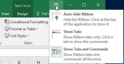
The Ribbon is designed to respond to your current task, but you can choose to minimize it if you find that it takes up too much screen space. Click the Ribbon Display Options arrow in the upper-right corner of the Ribbon to display the drop-down menu.
There are three modes in the Ribbon Display Options menu:
- Auto-hide Ribbon: Auto-hide displays your workbook in full-screen mode and completely hides the Ribbon. To show the Ribbon, click the Expand Ribbon command at the top of screen.
- Show Tabs: This option hides all command groups when they're not in use, but tabs will remain visible. To show the Ribbon, simply click a tab.
- Show Tabs and Commands: This option maximizes the Ribbon. All of the tabs and commands will be visible. This option is selected by default when you open Excel for the first time.
The Quick Access Toolbar
Located just above the Ribbon, the Quick Access Toolbar lets you access common commands no matter which tab is selected. By default, it includes the Save, Undo, and Repeat commands. You can add other commands depending on your preference.
To add commands to the Quick Access Toolbar:
- Click the drop-down arrow to the right of the Quick Access Toolbar.
- Select the command you want to add from the drop-down menu. To choose from more commands, select More Commands.
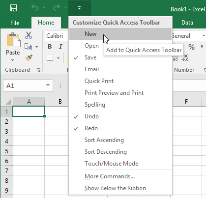
- The command will be added to the Quick Access Toolbar.
How to use Tell me:
The Tell me box works like a search bar to help you quickly find tools or commands you want to use.
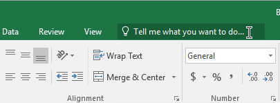
- Type in your own words what you want to do.
- The results will give you a few relevant options. To use one, click it like you would a command on the Ribbon.
Worksheet views
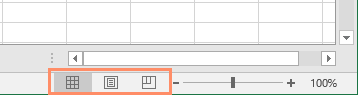
Excel 2016 has a variety of viewing options that change how your workbook is displayed. These views can be useful for various tasks, especially if you're planning to print the spreadsheet. To change worksheet views, locate the commands in the bottom-right corner of the Excel window and select Normal view, Page Layout view, or Page Break view.
- Normal view is the default view for all worksheets in Excel.
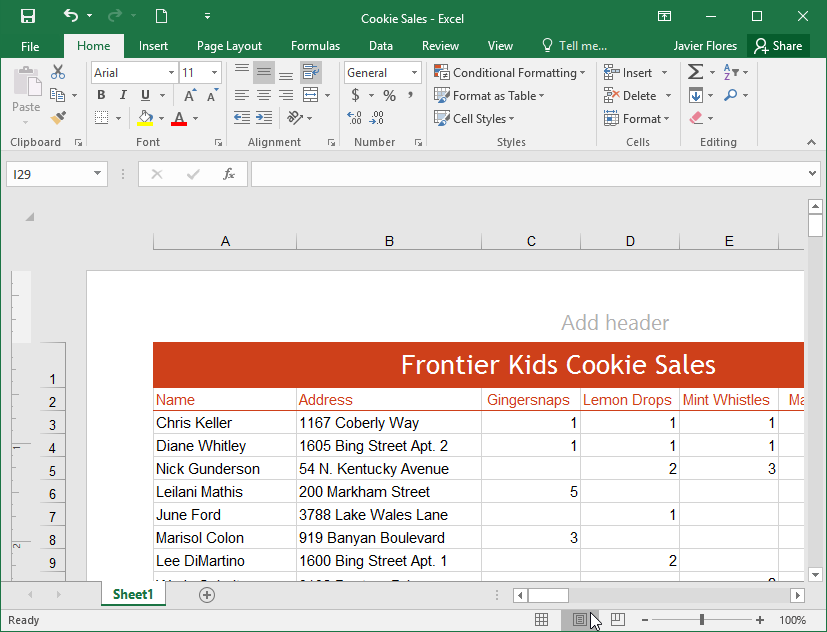
- Page Layout view displays how your worksheets will appear when printed. You can also add headers and footers in this view.
- Page Break view allows you to change the location of page breaks, which is especially helpful when printing a lot of data from Excel.
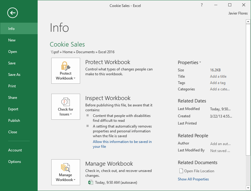
Backstage view
Backstage view gives you various options for saving, opening a file, printing, and sharing your workbooks.
To access Backstage view:
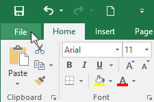
- Click the File tab on the Ribbon. Backstage view will appear.

Click the buttons in the interactive below to learn more about using Backstage view.
Challenge!
- Open Excel 2016.
- Click Blank Workbook to open a new spreadsheet.
- Change the Ribbon Display Options to Show Tabs.
- Using the Customize Quick Access Toolbar, click to add New, Quick Print, and Spelling.
- In the Tell me bar, type the word Color. Hover over Fill Color and choose a yellow. This will fill a cell with the color yellow.
- Change the worksheet view to the Page Layout option.
- When you're finished, your screen should look like this:
- Change the Ribbon Display Options back to Show Tabs and Commands.
- Close Excel and Don't Save changes.
Lesson 2: Understanding OneDrive
Introduction
Many of the features in Office are geared toward saving and sharing files online. OneDrive is Microsoft’s online storage space you can use to save, edit, and share your documents and other files. You can access OneDrive from your computer, smartphone, or any of the devices you use.
To get started with OneDrive, all you need to do is set up a free Microsoft account, if you don’t already have one.
If you don't already have a Microsoft account, you can go to the Creating a Microsoft Account lesson in our Microsoft Account tutorial.
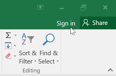
Once you have a Microsoft account, you'll be able to sign in to Office. Just click Sign in in the upper-right corner of the Excel window.
Benefits of using OneDrive
Once you’re signed in to your Microsoft account, here are a few of the things you’ll be able to do with OneDrive:
- Access your files anywhere: When you save your files to OneDrive, you’ll be able to access them from any computer, tablet, or smartphone that has an Internet connection. You'll also be able to create new documents from OneDrive.
- Back up your files: Saving files to OneDrive gives them an extra layer of protection. Even if something happens to your computer, OneDrive will keep your files safe and accessible.
- Share files: It’s easy to share your OneDrive files with friends and coworkers. You can choose whether they can edit or simply read files. This option is great for collaboration because multiple people can edit a document at the same time (this is also known as co-authoring).
Saving and opening files
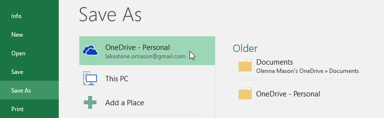
When you’re signed in to your Microsoft account, OneDrive will appear as an option whenever you save or open a file. You still have the option of saving files to your computer. However, saving files to your OneDrive allows you to access them from any other computer, and it also allows you to share files with friends and coworkers.
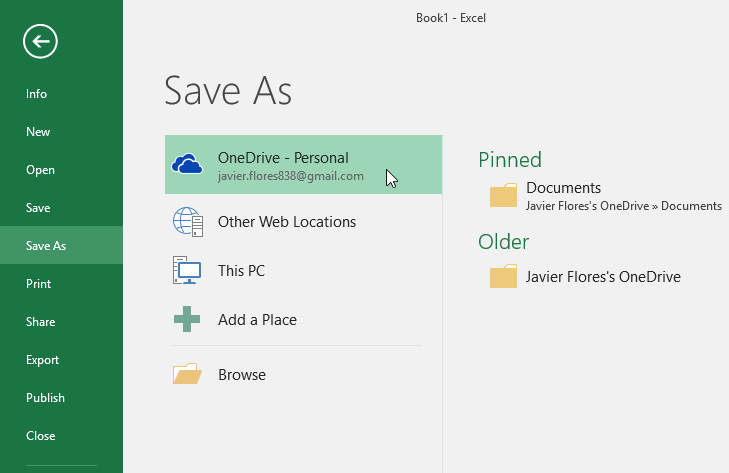
For example, when you click Save As, you can select either OneDrive or This PC as the save location.
Lesson 3: Creating and Opening Workbooks
Introduction
Excel files are called workbooks. Whenever you start a new project in Excel, you'll need to create a new workbook. There are several ways to start working with a workbook in Excel. You can choose to create a new workbook—either with a blank workbook or a predesigned template—or open an existing workbook.
Watch the video below to learn more about creating and opening workbooks in Excel.
About OneDrive
Whenever you're opening or saving a workbook, you'll have the option of using your OneDrive, which is the online file storage service included with your Microsoft account. To enable this option, you'll need to sign in to Office. To learn more, visit our lesson on Understanding OneDrive.
To create a new blank workbook:
- Select the File tab. Backstage view will appear.
- Select New, then click Blank workbook.
- A new blank workbook will appear.
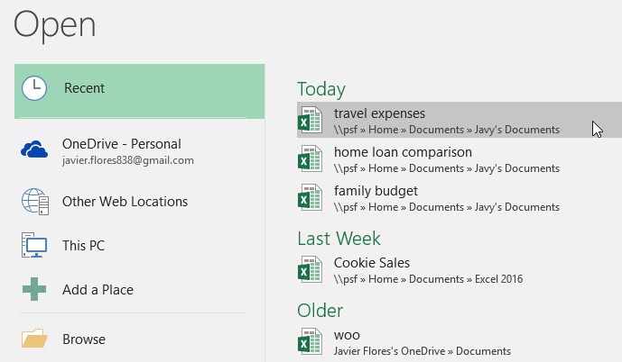
To open an existing workbook:
In addition to creating new workbooks, you'll often need to open a workbook that was previously saved. To learn more about saving workbooks, visit our lesson on Saving and Sharing Workbooks.
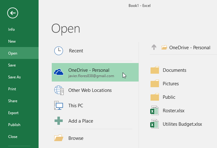
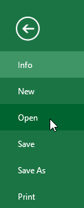
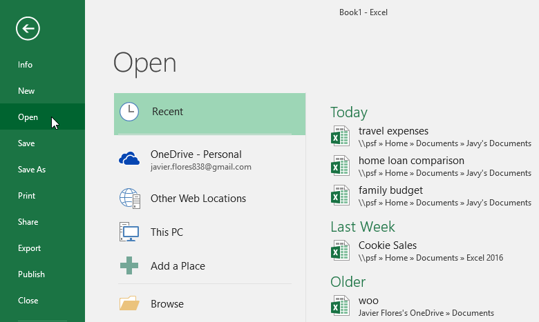
- Navigate to Backstage view, then click Open.
- Select Computer, then click Browse. Alternatively, you can choose OneDrive to open files stored on your OneDrive.
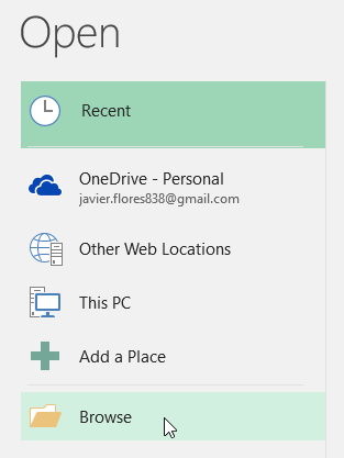
- The Open dialog box will appear. Locate and select your workbook, then click Open.
If you've opened the desired workbook recently, you can browse your Recent Workbooks rather than search for the file.
To pin a workbook:
If you frequently work with the same workbook, you can pin it to Backstage view for faster access.
- Navigate to Backstage view, then click Open. Your recently edited workbooks will appear.
- Hover the mouse over the workbook you want to pin. A pushpin icon will appear next to the workbook. Click the pushpin icon.
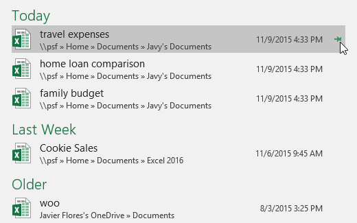
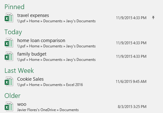
- The workbook will stay in Recent Workbooks. To unpin a workbook, simply click the pushpin icon again.
Using templates
A template is a predesigned spreadsheet you can use to create a new workbook quickly. Templates often include custom formatting and predefined formulas, so they can save you a lot of time and effort when starting a new project.
To create a new workbook from a template:
- Click the File tab to access Backstage view.
- Select New. Several templates will appear below the Blank workbook option.
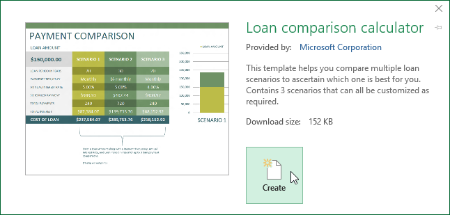
- Select a template to review it.
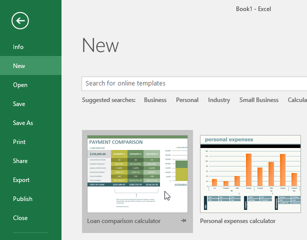
- A preview of the template will appear, along with additional information on how the template can be used.
- Click Create to use the selected template.
- A new workbook will appear with the selected template.
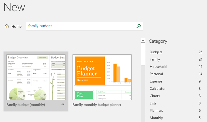
You can also browse templates by category or use the search bar to find something more specific.
It's important to note that not all templates are created by Microsoft. Many are created by third-party providers and even individual users, so some templates may work better than others.
Compatibility Mode
Sometimes you may need to work with workbooks that were created in earlier versions of Microsoft Excel, such as Excel 2003 or Excel 2000. When you open these types of workbooks, they will appear in Compatibility Mode.
Compatibility Mode disables certain features, so you'll only be able to access commands found in the program that was used to create the workbook. For example, if you open a workbook created in Excel 2003, you can only use tabs and commands found in Excel 2003.
In the image below, you can see that the workbook is in Compatibility Mode, which is indicated at the top of the window to the right of the file name. This will disable some Excel 2016 features, and they will be grayed out on the Ribbon.
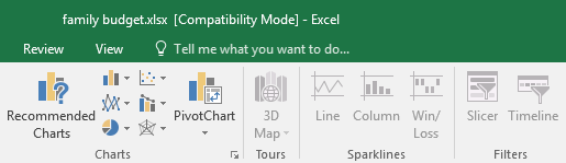
In order to exit Compatibility Mode, you'll need to convert the workbook to the current version type. However, if you're collaborating with others who only have access to an earlier version of Excel, it's best to leave the workbook in Compatibility Mode so the format will not change.
To convert a workbook:
If you want access to all of the Excel 2016 features, you can convert the workbook to the 2016 file format.
Note that converting a file may cause some changes to the original layout of the workbook.
- Click the File tab to access Backstage view.
- Locate and select Convert command.

- The Save As dialog box will appear. Select the location where you want to save the workbook, enter a file name for the workbook, and click Save.
- The workbook will be converted to the newest file type.
Challenge!
- Open our practice workbook.
- Notice that our workbook opens in Compatibility Mode. Convert the workbook to the 2016 file format. A dialog box will appear asking if you would like to close and reopen the file in order to see the new features. Choose Yes.
- Lastly, in the Backstage view, pin a file or folder.
Lesson 4: Saving and Sharing Workbooks
Introduction
Whenever you create a new workbook in Excel, you'll need to know how to save it in order to access and edit it later. As with previous versions of Excel, you can save files locally to your computer. But unlike older versions, Excel 2016 also lets you save a workbook to the cloud using OneDrive. You can also export and share workbooks with others directly from Excel.
Watch the video below to learn more about saving and sharing workbooks in Excel.
About OneDrive
Whenever you're opening or saving a workbook, you'll have the option of using your OneDrive, which is the online file storage service included with your Microsoft account. To enable this option, you'll need to sign in to Office. To learn more, visit our lesson on Understanding OneDrive.
Save and Save As
Excel offers two ways to save a file: Save and Save As. These options work in similar ways, with a few important differences:
- Save: When you create or edit a workbook, you'll use the Save command to save your changes. You'll use this command most of the time. When you save a file, you'll only need to choose a file name and location the first time. After that, you can just click the Save command to save it with the same name and location.
- Save As: You'll use this command to create a copy of a workbook while keeping the original. When you use Save As, you'll need to choose a different name and/or location for the copied version.
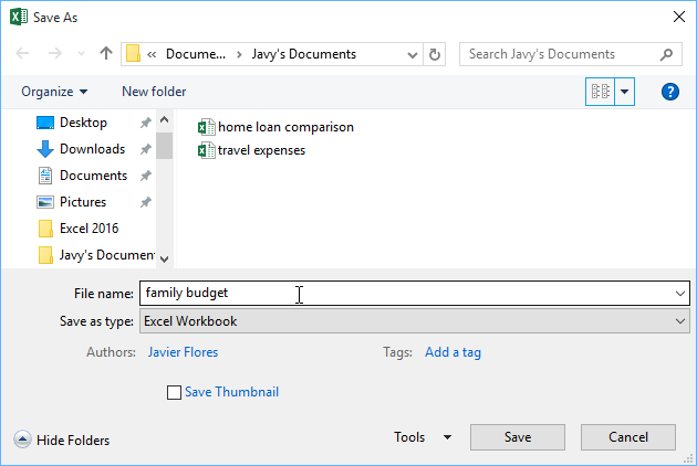
To save a workbook:
It's important to save your workbook whenever you start a new project or make changes to an existing one. Saving early and often can prevent your work from being lost. You'll also need to pay close attention to where you save the workbook so it will be easy to find later.
- Locate and select the Save command on the Quick Access Toolbar.
- If you're saving the file for the first time, the Save As pane will appear in Backstage view.
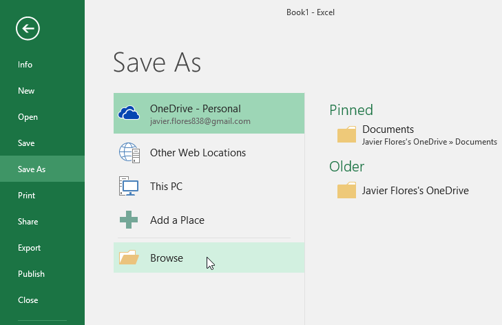
- You'll then need to choose where to save the file and give it a file name. To save the workbook to your computer, select Computer, then click Browse. Alternatively, you can click OneDrive to save the file to your OneDrive.
- The Save As dialog box will appear. Select the location where you want to save the workbook.
- Enter a file name for the workbook, then click Save.
- The workbook will be saved. You can click the Save command again to save your changes as you modify the workbook.
You can also access the Save command by pressing Ctrl+S on your keyboard.
Using Save As to make a copy
If you want to save a different version of a workbook while keeping the original, you can create a copy. For example, if you have a file named Sales Data, you could save it as Sales Data 2 so you'll be able to edit the new file and still refer back to the original version.
To do this, you'll click the Save As command in Backstage view. Just like when saving a file for the first time, you'll need to choose where to save the file and give it a new file name.
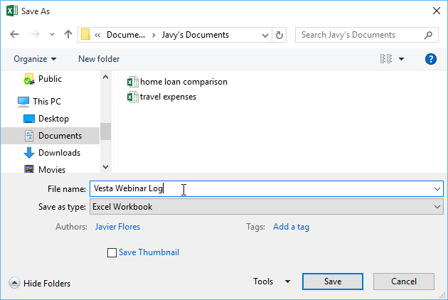
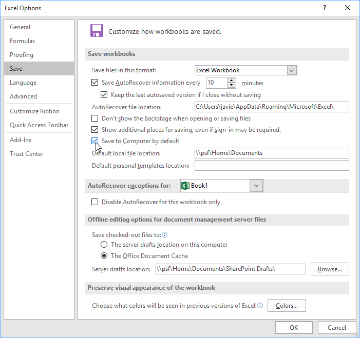
To change the default save location:
If you don't want to use OneDrive, you may be frustrated that OneDrive is selected as the default location when saving. If you find it inconvenient to select Computer each time, you can change the default save location so Computer is selected by default.
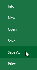
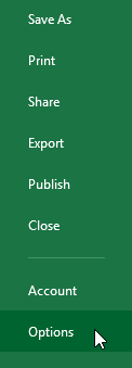
- Click the File tab to access Backstage view.

- Click Options.
- The Excel Options dialog box will appear. Select Save, check the box next to Save to Computer by default, then click OK. The default save location will be changed.
AutoRecover
Excel automatically saves your workbooks to a temporary folder while you are working on them. If you forget to save your changes or if Excel crashes, you can restore the file using AutoRecover.
To use AutoRecover:
- Open Excel. If autosaved versions of a file are found, the Document Recovery pane will appear.
- Click to open an available file. The workbook will be recovered.
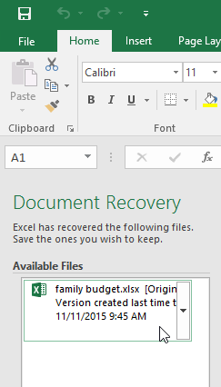
By default, Excel autosaves every 10 minutes. If you are editing a workbook for less than 10 minutes, Excel may not create an autosaved version.
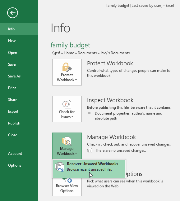
If you don't see the file you need, you can browse all autosaved files from Backstage view. Just select the File tab, click Manage Versions, then choose Recover Unsaved Workbooks.
Exporting workbooks
By default, Excel workbooks are saved in the .xlsx file type. However, there may be times when you need to use another file type, such as a PDF or Excel 97-2003 workbook. It's easy to export your workbook from Excel to a variety of file types.
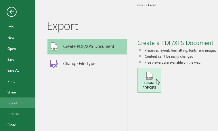
To export a workbook as a PDF file:
Exporting your workbook as an Adobe Acrobat document, commonly known as a PDF file, can be especially useful if you're sharing a workbook with someone who does not have Excel. A PDF will make it possible for recipients to view but not edit the content of your workbook.
- Click the File tab to access Backstage view.
- Click Export, then select Create PDF/XPS.
- The Save As dialog box will appear. Select the location where you want to export the workbook, enter a file name, then click Publish.
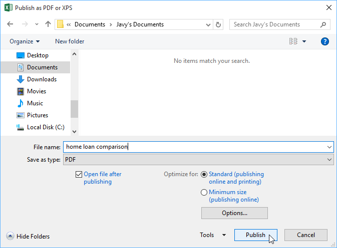
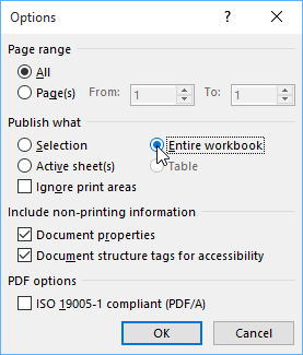
By default, Excel will only export the active worksheet. If you have multiple worksheets and want to save all of them in the same PDF file, click Options in the Save As dialog box. The Options dialog box will appear. Select Entire workbook, then click OK.
Whenever you export a workbook as a PDF, you'll also need to consider how your workbook data will appear on each page of the PDF, just like printing a workbook. Visit our Page Layout and Printing lesson to learn more about what to consider before exporting a workbook as a PDF.
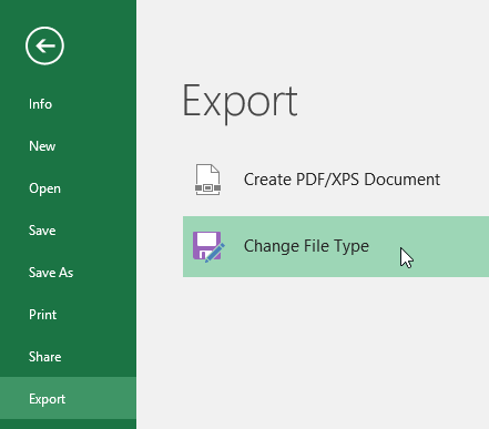
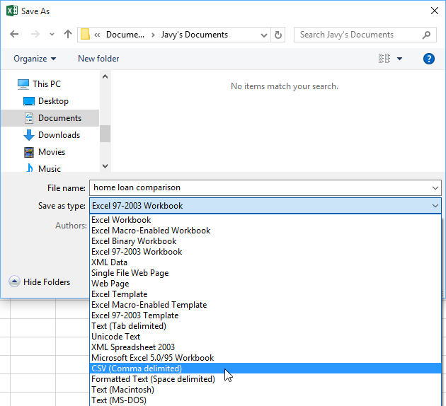
To export a workbook to other file types:
You may also find it helpful to export your workbook to other file types, such as an Excel 97-2003 workbook if you need to share with people using an older version of Excel, or a .CSV file if you need a plain-text version of your workbook.
- Click the File tab to access Backstage view.
- Click Export, then select Change File Type.
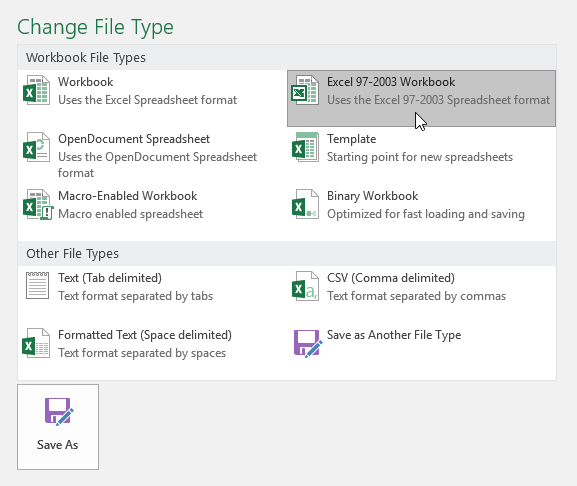
- Select a common file type, then click Save As.
- The Save As dialog box will appear. Select the location where you want to export the workbook, enter a file name, then click Save.
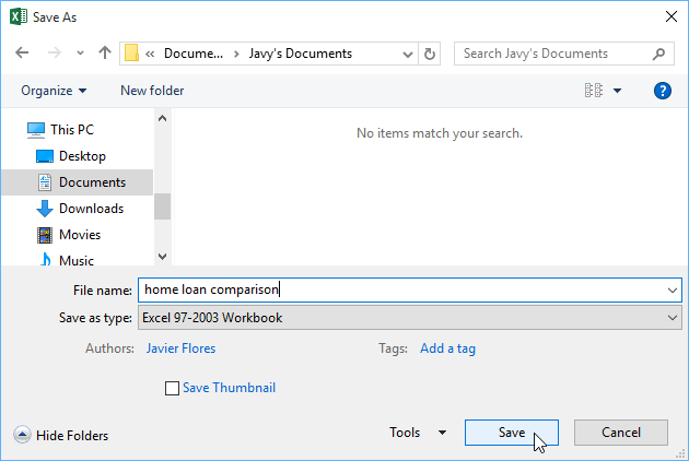
You can also use the Save as type: drop-down menu in the Save As dialog box to save workbooks in a variety of file types.
Sharing workbooks
Excel makes it easy to share and collaborate on workbooks using OneDrive. In the past, if you wanted to share a file with someone you could send it as an email attachment. While convenient, this system also creates multiple versions of the same file, which can be difficult to organize.
When you share a workbook from Excel, you're actually giving others access to the exact same file. This lets you and the people you share with edit the same workbook without having to keep track of multiple versions.
In order to share a workbook, it must first be saved to your OneDrive.
To share a workbook:
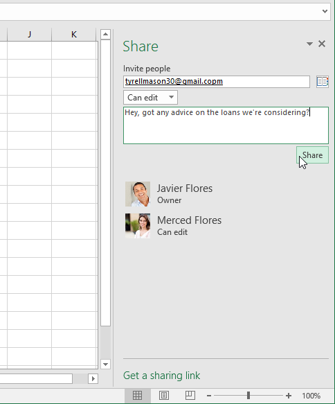
- Click the File tab to access Backstage view, then click Share.
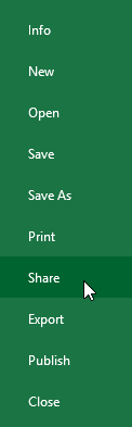
- The Share pane will appear. If you have not already done so, you will be prompted to save your document to OneDrive. Note that you may need to navigate back to the Share pane after saving.
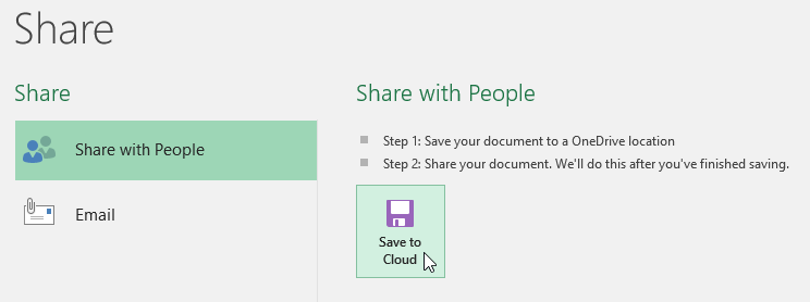
- On the Share pane, if your document is saved to OneDrive, click the Share with People button.
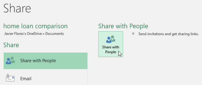
- Excel will return to Normal view and open the Share panel on the right side of the window. From here, you can invite people to share your document, see a list of who has access to the document, and set whether they can edit or only view the document.
Challenge!
- Open our practice workbook.
- Using the Save As option, create a copy of the workbook and name it Saving Practice Challenge. You can save the copy to a folder on your computer or to your OneDrive.
- Export the workbook as a PDF file.
Lesson 5: Cell Basics
Introduction
Whenever you work with Excel, you'll enter information—or content—into cells. Cells are the basic building blocks of a worksheet. You'll need to learn the basics of cells and cell content to calculate, analyze, and organize data in Excel.
Optional: Download our practice workbook.
Watch the video below to learn more about the basics of working with cells.
Understanding cells
Every worksheet is made up of thousands of rectangles, which are called cells. A cell is the intersection of a row and a column—in other words, where a row and column meet.
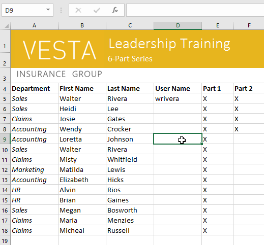
Columns are identified by letters (A, B, C), while rows are identified by numbers (1, 2, 3). Each cell has its own name—or cell address—based on its column and row. In the example below, the selected cell intersects column C and row 5, so the cell address is C5.
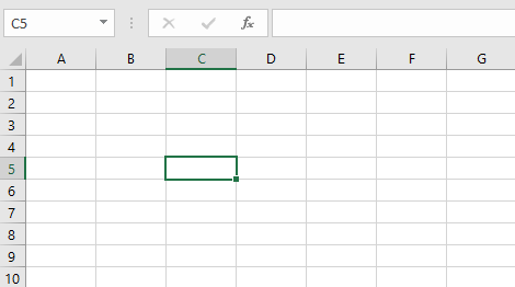
Note that the cell address also appears in the Name box in the top-left corner, and that a cell's column and row headings are highlighted when the cell is selected.
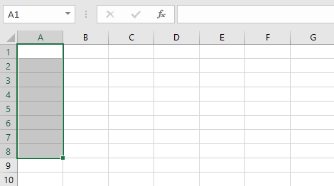
You can also select multiple cells at the same time. A group of cells is known as a cell range. Rather than a single cell address, you will refer to a cell range using the cell addresses of the first and last cells in the cell range, separated by a colon. For example, a cell range that included cells A1, A2, A3, A4, and A5 would be written as A1:A5. Take a look at the different cell ranges below:
- Cell range A1:A8
- Cell range A1:F1
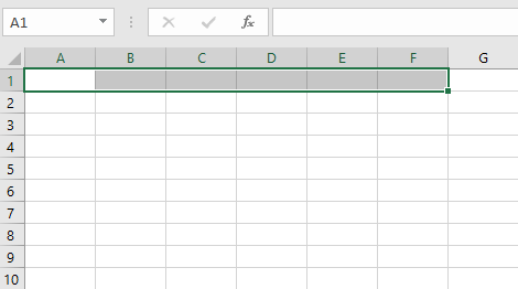
- Cell range A1:F8
If the columns in your spreadsheet are labeled with numbers instead of letters, you'll need to change the default reference style for Excel. Review our Extra on What are Reference Styles? to learn how.
To select a cell:
To input or edit cell content, you'll first need to select the cell.
- Click a cell to select it. In our example, we'll select cell D9.
- A border will appear around the selected cell, and the column heading and row heading will be highlighted. The cell will remain selected until you click another cell in the worksheet.
You can also select cells using the arrow keys on your keyboard.
To select a cell range:
Sometimes you may want to select a larger group of cells, or a cell range.
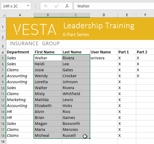
- Click and drag the mouse until all of the adjoining cells you want to select are highlighted. In our example, we'll select the cell range B5:C18.
- Release the mouse to select the desired cell range. The cells will remain selected until you click another cell in the worksheet.
Cell content
Any information you enter into a spreadsheet will be stored in a cell. Each cell can contain different types of content, including text, formatting, formulas, and functions.
- Text: Cells can contain text, such as letters, numbers, and dates.
- Formatting attributes: Cells can contain formatting attributes that change the way letters, numbers, and dates are displayed. For example, percentages can appear as 0.15 or 15%. You can even change a cell's text or background color.
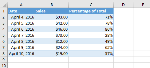
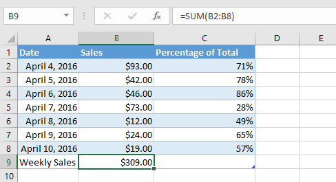
- Formulas and functions: Cells can contain formulas and functions that calculate cell values. In our example, SUM(B2:B8) adds the value of each cell in the cell range B2:B8 and displays the total in cell B9.
To insert content:
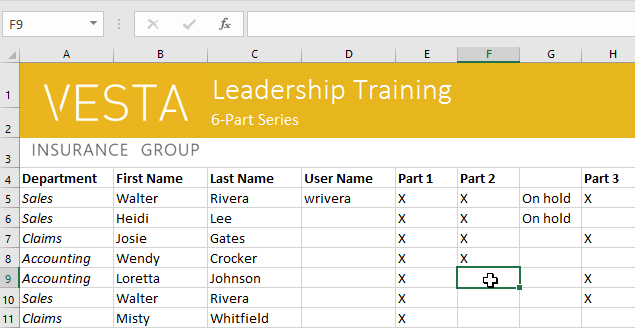
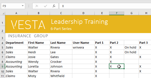
- Click a cell to select it. In our example, we'll select cell F9.
- Type something into the selected cell, then press Enter on your keyboard. The content will appear in the cell and the formula bar. You can also input and edit cell content in the formula bar.
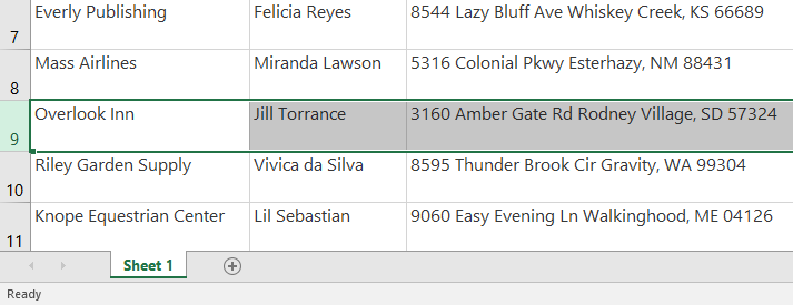
To delete (or clear) cell content:
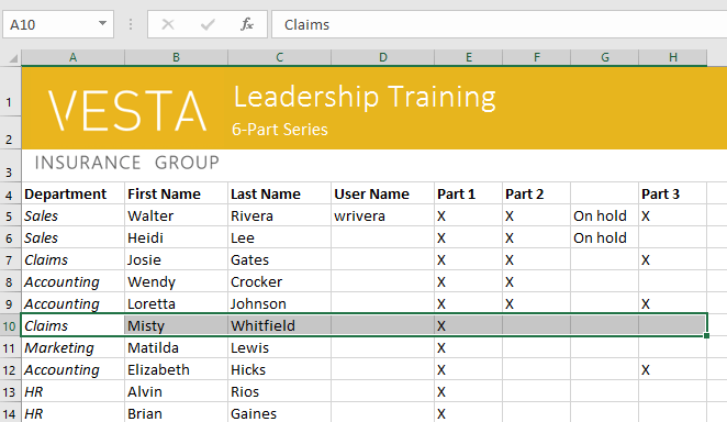
- Select the cell(s) with content you want to delete. In our example, we'll select the cell range A10:H10.
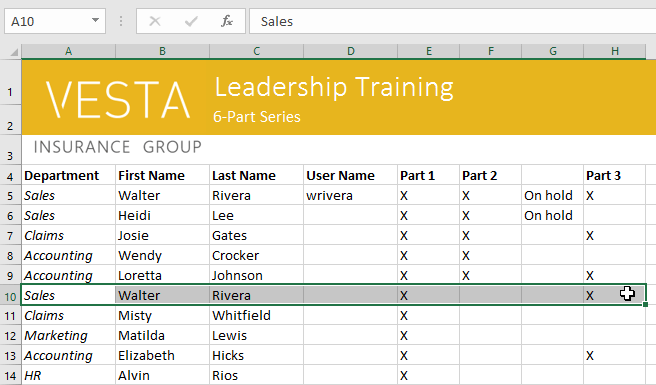
- Select the Clear command on the Home tab, then click Clear Contents.
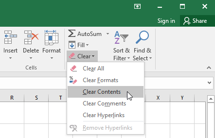
- The cell contents will be deleted.
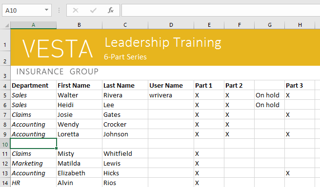
You can also use the Delete key on your keyboard to delete content from multiple cells at once. The Backspace key will only delete content from one cell at a time.
To delete cells:
There is an important difference between deleting the content of a cell and deleting the cell itself. If you delete the entire cell, the cells below it will shift to fill in the gaps and replace the deleted cells.
- Select the cell(s) you want to delete. In our example, we'll select A10:H10.
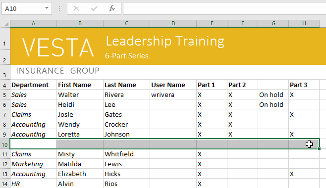
- Select the Delete command from the Home tab on the Ribbon.
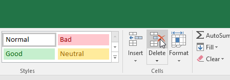
- The cells below will shift up and fill in the gaps.
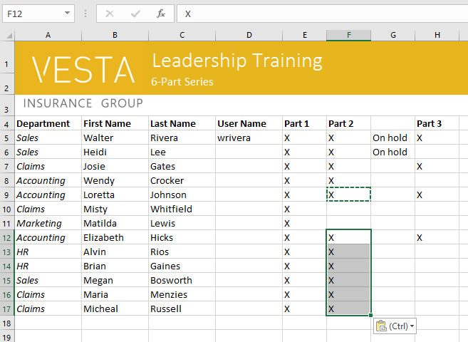
To copy and paste cell content:
Excel allows you to copy content that is already entered into your spreadsheet and paste that content to other cells, which can save you time and effort.
- Select the cell(s) you want to copy. In our example, we'll select F9.
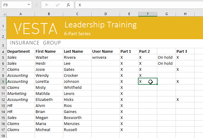
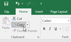
- Click the Copy command on the Home tab, or press Ctrl+C on your keyboard.
- Select the cell(s) where you want to paste the content. In our example, we'll select F12:F17. The copied cell(s) will have a dashed box around them.
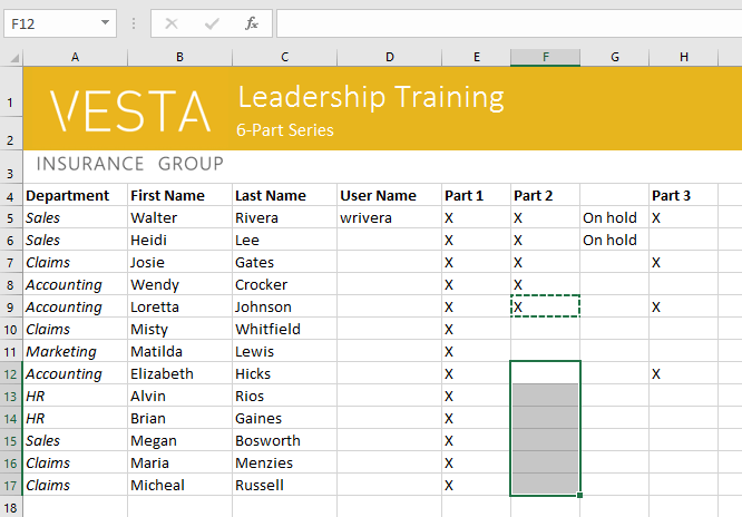
- Click the Paste command on the Home tab, or press Ctrl+V on your keyboard.
- The content will be pasted into the selected cells.
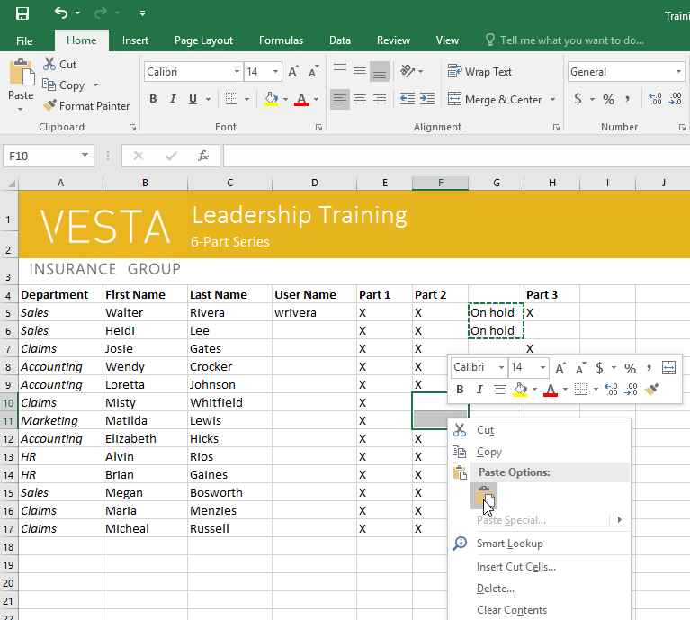
To access more paste options:
You can also access additional paste options, which are especially convenient when working with cells that contain formulas or formatting. Just click the drop-down arrow on the Paste command to see these options.
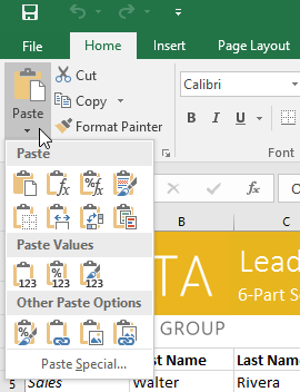
Instead of choosing commands from the Ribbon, you can access commands quickly by right-clicking. Simply select the cell(s) you want to format, then right-click the mouse. A drop-down menu will appear, where you'll find several commands that are also located on the Ribbon.
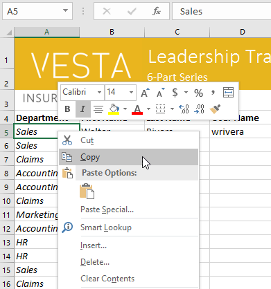
To cut and paste cell content:
Unlike copying and pasting, which duplicates cell content, cutting allows you to move content between cells.
- Select the cell(s) you want to cut. In our example, we'll select G5:G6.
- Right-click the mouse and select the Cut command. Alternatively, you can use the command on the Home tab, or press Ctrl+X on your keyboard.
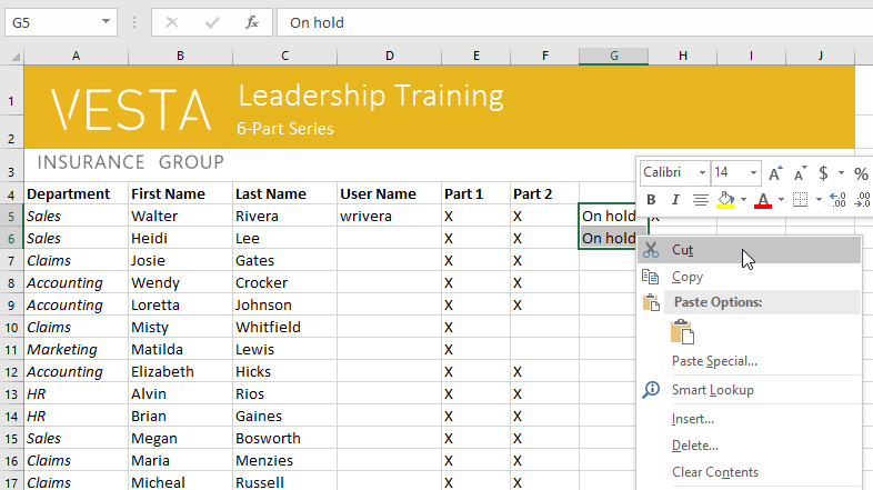
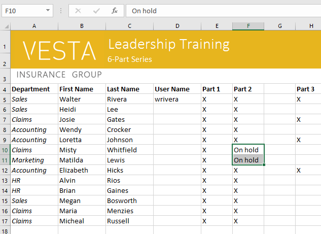
- Select the cells where you want to paste the content. In our example, we'll select F10:F11. The cut cells will now have a dashed box around them.
- Right-click the mouse and select the Paste command. Alternatively, you can use the command on the Home tab, or press Ctrl+V on your keyboard.
- The cut content will be removed from the original cells and pasted into the selected cells.
To drag and drop cells:
Instead of cutting, copying, and pasting, you can drag and drop cells to move their contents.
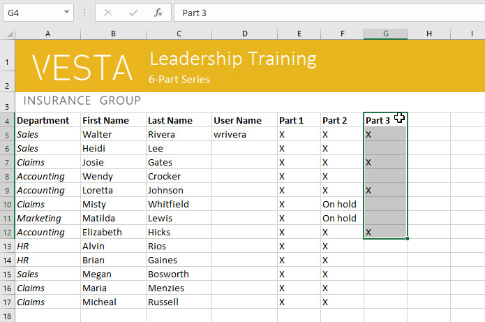
- Select the cell(s) you want to move. In our example, we'll select H4:H12.
- Hover the mouse over the border of the selected cell(s) until the mouse changes to a pointer with four arrows.
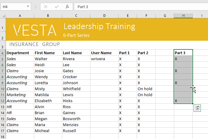
- Click and drag the cells to the desired location. In our example, we'll move them to G4:G12.
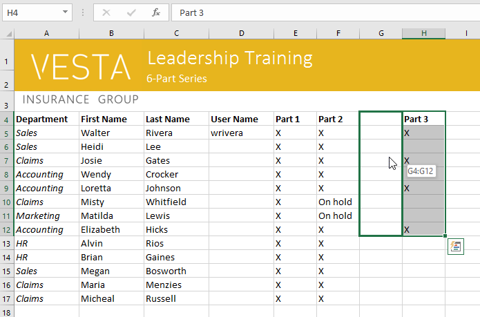
- Release the mouse. The cells will be dropped in the selected location.
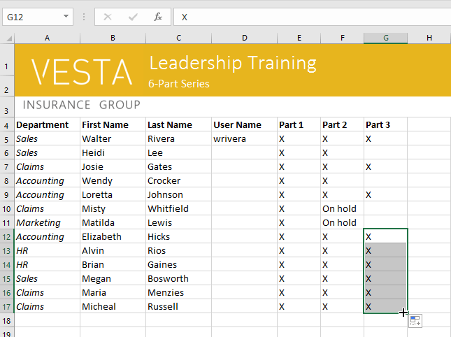
To use the fill handle:
If you're copying cell content to adjacent cells in the same row or column, the fill handle is a good alternative to the copy and paste commands.
- Select the cell(s) containing the content you want to use, then hover the mouse over the lower-right corner of the cell so the fill handle appears.
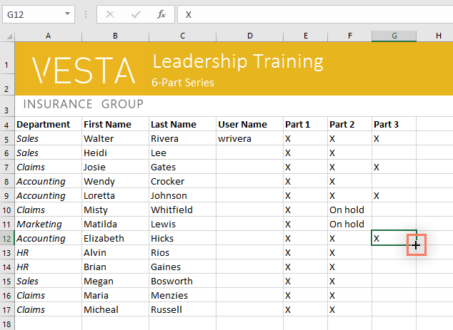
- Click and drag the fill handle until all of the cells you want to fill are selected. In our example, we'll select G13:G17.
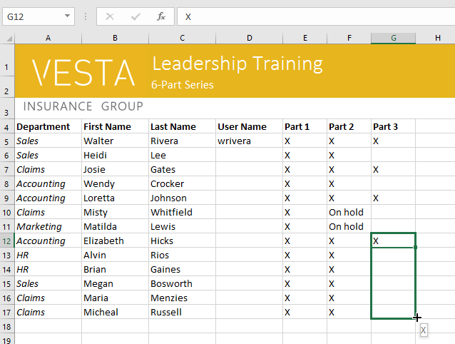
- Release the mouse to fill the selected cells.
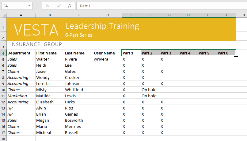
To continue a series with the fill handle:
The fill handle can also be used to continue a series. Whenever the content of a row or column follows a sequential order, like numbers (1, 2, 3) or days (Monday, Tuesday, Wednesday), the fill handle can guess what should come next in the series. In most cases, you will need to select multiple cells before using the fill handle to help Excel determine the series order. Let's take a look at an example:
- Select the cell range that contains the series you want to continue. In our example, we'll select E4:G4.
- Click and drag the fill handle to continue the series.
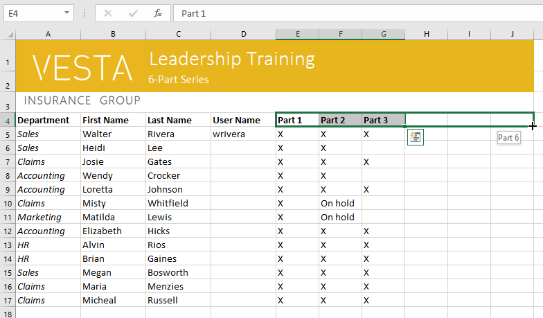
- Release the mouse. If Excel understood the series, it will be continued in the selected cells. In our example, Excel added Part 4, Part 5, and Part 6 to H4:J4.
You can also double-click the fill handle instead of clicking and dragging. This can be useful with larger spreadsheets, where clicking and dragging may be awkward.
Watch the video below to see an example of double-clicking the fill handle.
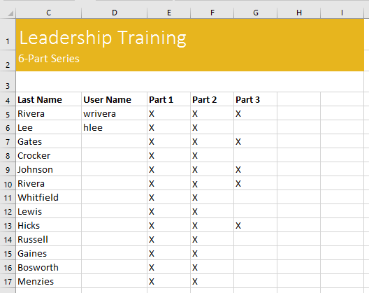
Challenge!
- Open our practice workbook.
- Select cell D6 and type hlee.
- Clear the contents in row 14.
- Delete column G.
- Using either cut and paste or drag and drop, move the contents of row 18 to row 14.
- Use the fill handle to put an X in cells F9:F17.
- When you're finished, your workbook should look like this:
Lesson 6: Modifying Columns, Rows, and Cells
Introduction
By default, every row and column of a new workbook is set to the same height and width. Excel allows you to modify column width and row height in different ways, including wrapping text and merging cells.
Optional: Download our practice workbook.
Watch the video below to learn more about modifying columns, rows, and cells.
To modify column width:
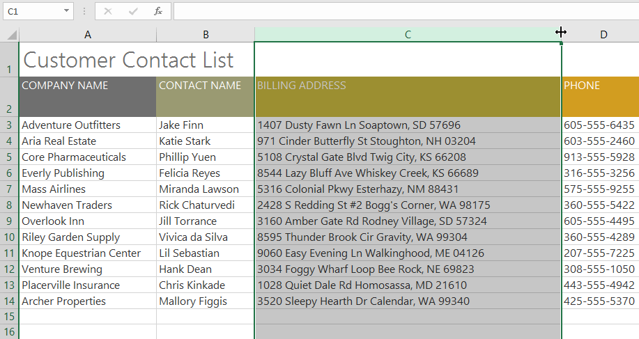
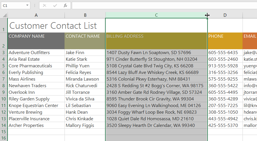
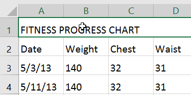
In our example below, column C is too narrow to display all of the content in these cells. We can make all of this content visible by changing the width of column C.
- Position the mouse over the column line in the column heading so the cursor becomes a double arrow.
- Click and drag the mouse to increase or decrease the column width.
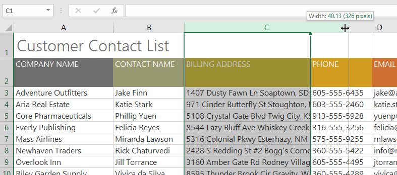
- Release the mouse. The column width will be changed.
With numerical data, the cell will display pound signs (#######) if the column is too narrow. Simply increase the column width to make the data visible.
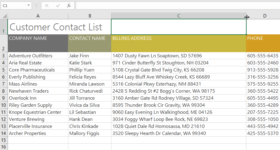
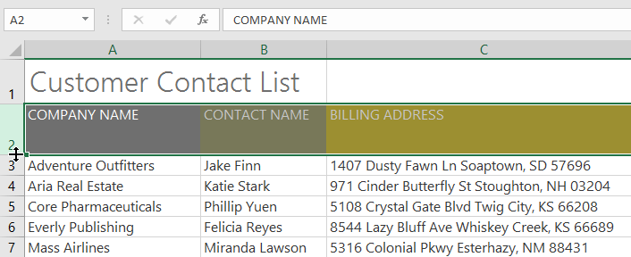
To AutoFit column width:
The AutoFit feature will allow you to set a column's width to fit its content automatically.
- Position the mouse over the column line in the column heading so the cursor becomes a double arrow.
- Double-click the mouse. The column width will be changed automatically to fit the content.
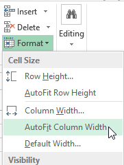
You can also AutoFit the width for several columns at the same time. Simply select the columns you want to AutoFit, then select the AutoFit Column Width command from the Format drop-down menu on the Home tab. This method can also be used for row height.
To modify row height:
- Position the cursor over the row line so the cursor becomes a double arrow.
- Click and drag the mouse to increase or decrease the row height.
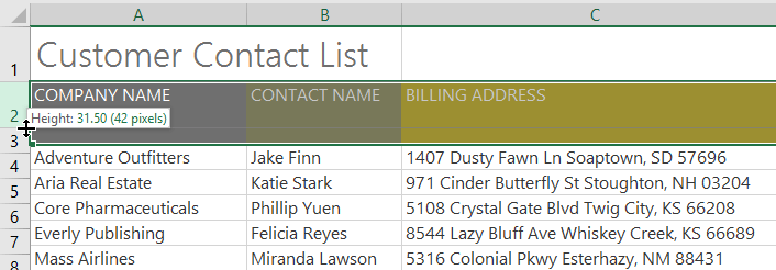
- Release the mouse. The height of the selected row will be changed.
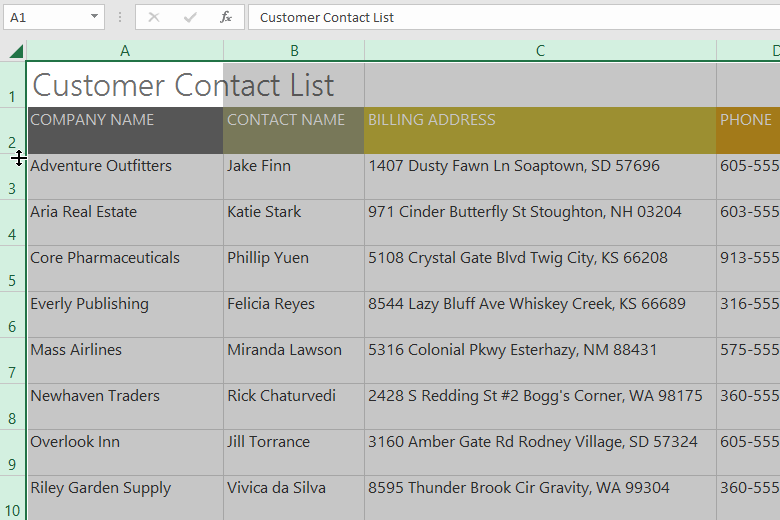
To modify all rows or columns:
Instead of resizing rows and columns individually, you can modify the height and width of every row and column at the same time. This method allows you to set a uniform size for every row and column in your worksheet. In our example, we will set a uniform row height.
- Locate and click the Select All button just below the name box to select every cell in the worksheet.

- Position the mouse over a row line so the cursor becomes a double arrow.
- Click and drag the mouse to increase or decrease the row height, then release the mouse when you are satisfied. The row height will be changed for the entire worksheet.
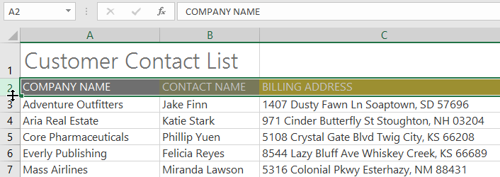
Inserting, deleting, moving, and hiding
After you've been working with a workbook for a while, you may find that you want to insert new columns or rows, delete certain rows or columns, move them to a different location in the worksheet, or even hide them.
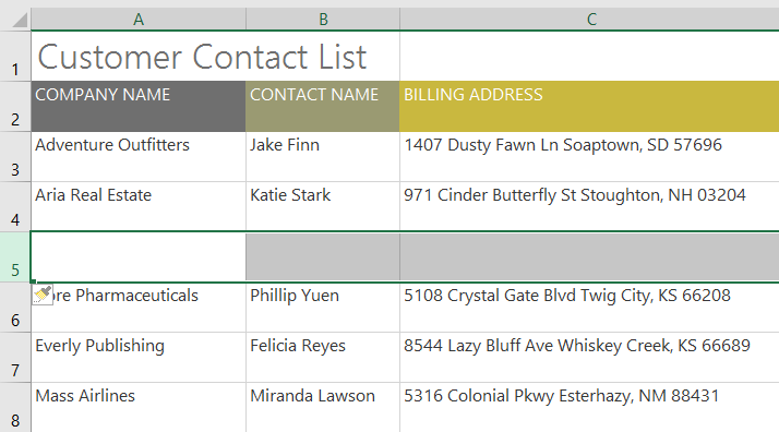
To insert rows:
- Select the row heading below where you want the new row to appear. In this example, we want to insert a row between rows 4 and 5, so we'll select row 5.
- Click the Insert command on the Home tab.
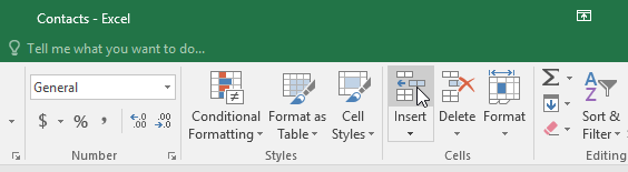
- The new row will appear above the selected row.
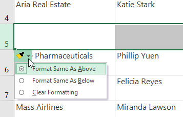
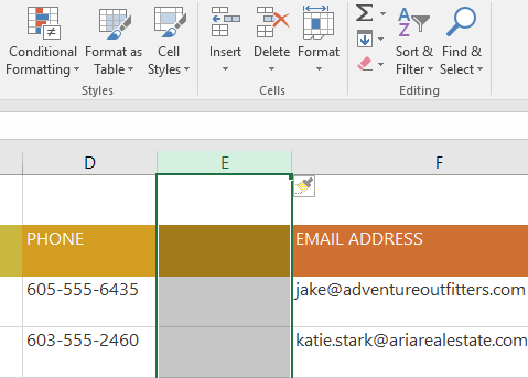
When inserting new rows, columns, or cells, you will see a paintbrush icon next to the inserted cells. This button allows you to choose how Excel formats these cells. By default, Excel formats inserted rows with the same formatting as the cells in the row above. To access more options, hover your mouse over the icon, then click the drop-down arrow.
To insert columns:
- Select the column heading to the right of where you want the new column to appear. For example, if you want to insert a column between columns D and E, select column E.
- Click the Insert command on the Home tab.
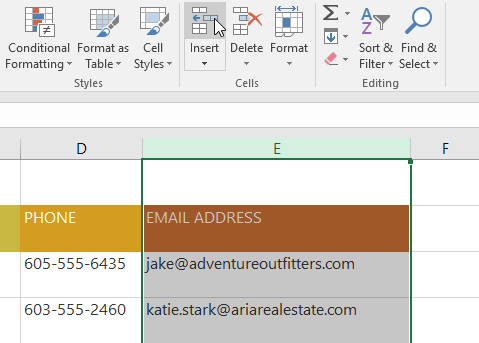
- The new column will appear to the left of the selected column.
When inserting rows and columns, make sure you select the entire row or column by clicking the heading. If you select only a cell in the row or column, the Insert command will only insert a new cell.
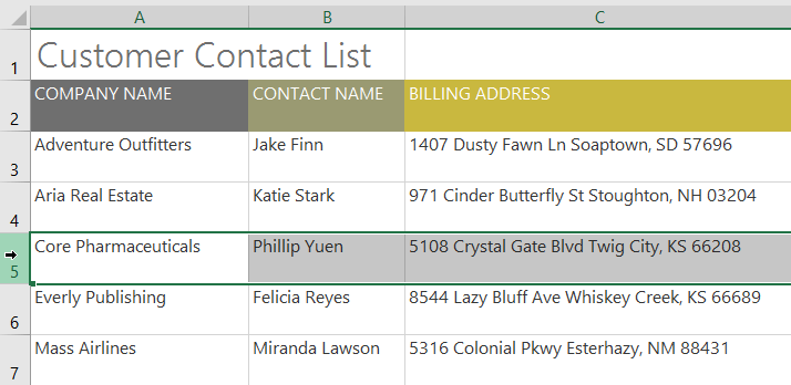
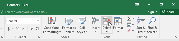
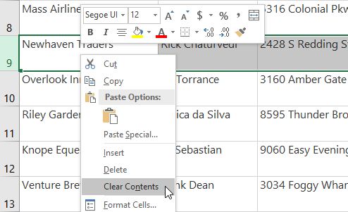
To delete a row or column:
It's easy to delete a row or column that you no longer need. In our example we'll delete a row, but you can delete a column the same way.
- Select the row you want to delete. In our example, we'll select row 9.
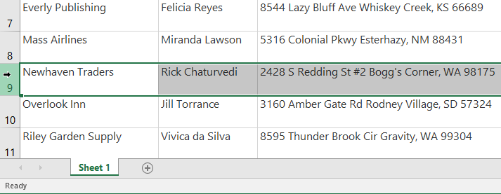
- Click the Delete command on the Home tab.
- The selected row will be deleted, and those around it will shift. In our example, row 10 has moved up, so it's now row 9.
It's important to understand the difference between deleting a row or column and simply clearing its contents. If you want to remove the content from a row or column without causing others to shift, right-click a heading, then select Clear Contents from the drop-down menu.
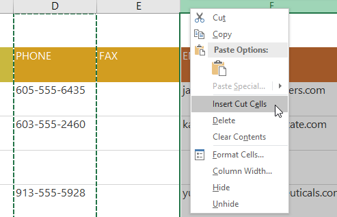
To move a row or column:
Sometimes you may want to move a column or row to rearrange the content of your worksheet. In our example we'll move a column, but you can move a row in the same way.
- Select the desired column heading for the column you want to move.
- Click the Cut command on the Home tab, or press Ctrl+X on your keyboard.
- Select the column heading to the right of where you want to move the column. For example, if you want to move a column between columns E and F, select column F.
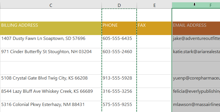
- Click the Insert command on the Home tab, then select Insert Cut Cells from the drop-down menu.
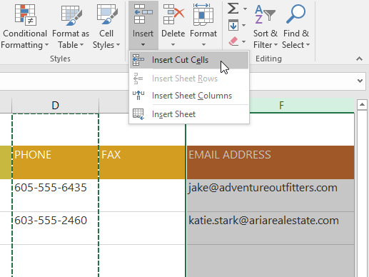
- The column will be moved to the selected location, and the columns around it will shift.
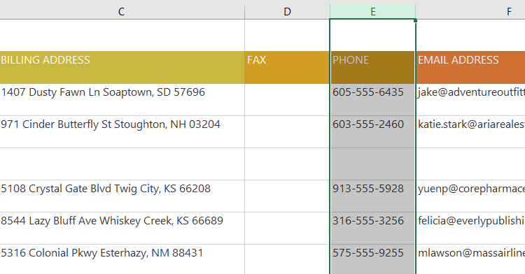
You can also access the Cut and Insert commands by right-clicking the mouse and selecting the desired commands from the drop-down menu.
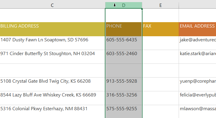
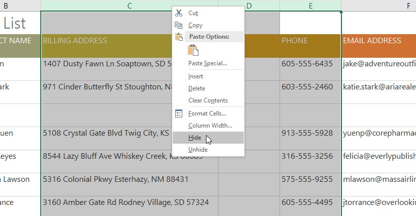
To hide and unhide a row or column:
At times, you may want to compare certain rows or columns without changing the organization of your worksheet. To do this, Excel allows you to hide rows and columns as needed. In our example we'll hide a few columns, but you can hide rows in the same way.
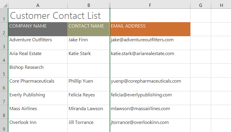
- Select the columns you want to hide, right-click the mouse, then select Hide from the formatting menu. In our example, we'll hide columns C, D, and E.
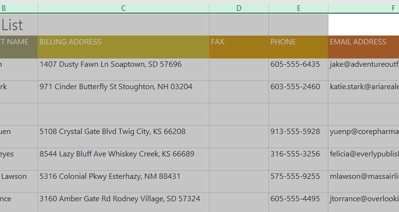
- The columns will be hidden. The green column line indicates the location of the hidden columns.
- To unhide the columns, select the columns on both sides of the hidden columns. In our example, we'll select columns B and F. Then right-click the mouse and select Unhide from the formatting menu.
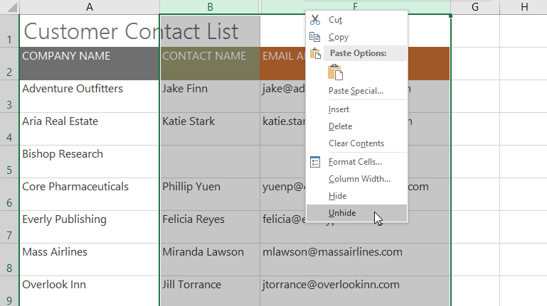
- The hidden columns will reappear.
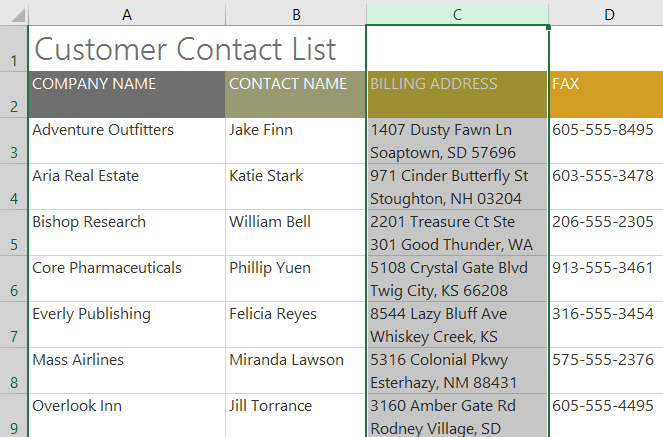
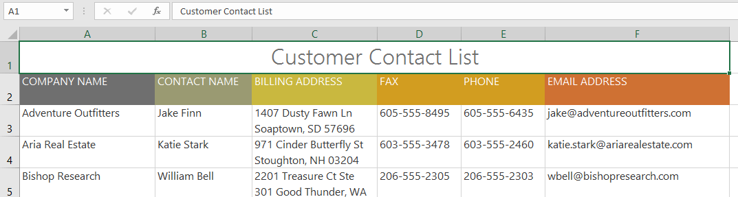
Wrapping text and merging cells
Whenever you have too much cell content to be displayed in a single cell, you may decide to wrap the text or merge the cell rather than resize a column. Wrapping the text will automatically modify a cell's row height, allowing cell contents to be displayed on multiple lines. Merging allows you to combine a cell with adjacent empty cells to create one large cell.
To wrap text in cells:
- Select the cells you want to wrap. In this example, we'll select the cells in column C.
- Click the Wrap Text command on the Home tab.
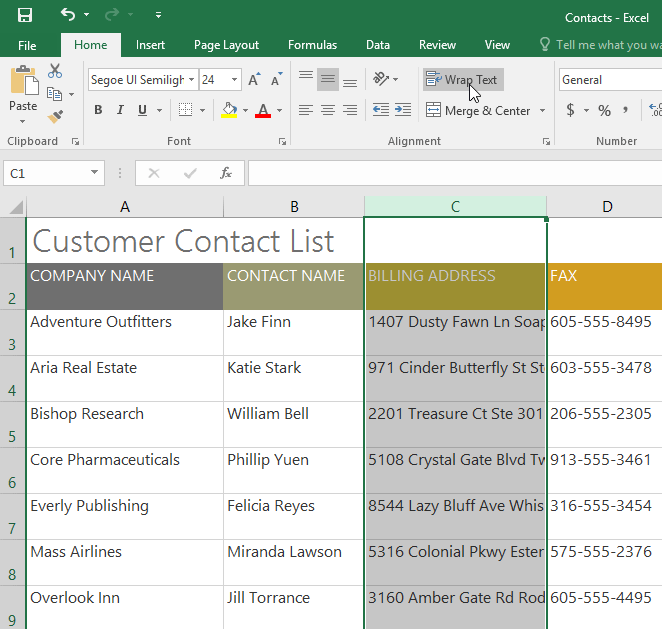
- The text in the selected cells will be wrapped.
Click the Wrap Text command again to unwrap the text.
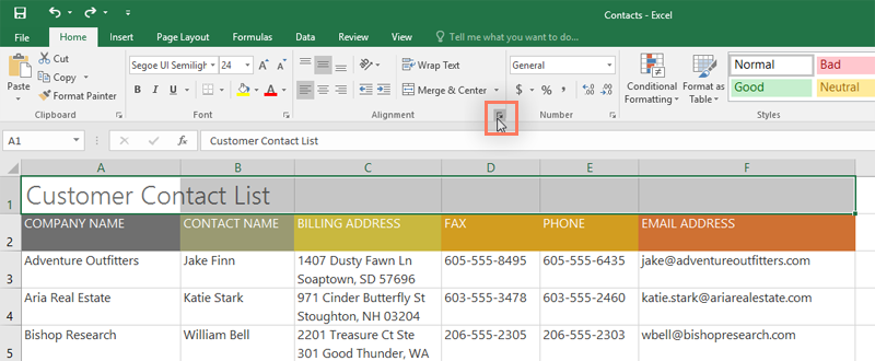
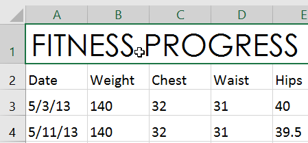
To merge cells using the Merge & Center command:
- Select the cell range you want to merge. In our example, we'll select A1:F1.
- Click the Merge & Center command on the Home tab. In our example, we'll select the cell range A1:F1.
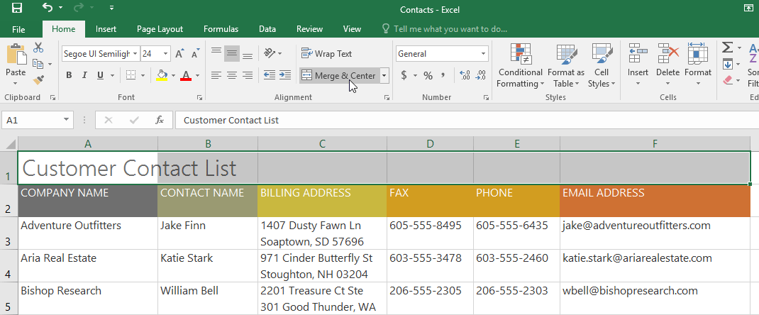
- The selected cells will be merged, and the text will be centered.
To access more merge options:
If you click the drop-down arrow next to the Merge & Center command on the Home tab, the Merge drop-down menu will appear.
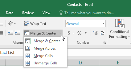
From here, you can choose to:
- Merge & Center: merges the selected cells into one cell and centers the text
- Merge Across: merges the selected cells into larger cells while keeping each row separate
- Merge Cells: merges the selected cells into one cell but does not center the text
- Unmerge Cells: unmerges selected cells
You'll want to be careful when using this feature. If you merge multiple cells that all contain data, Excel will keep only the contents of the upper-left cell and discard everything else.
To center across selection:
Merging can be useful for organizing your data, but it can also create problems later on. For example, it can be difficult to move, copy, and paste content from merged cells. A good alternative to merging is Center Across Selection, which creates a similar effect without actually combining cells.
Watch the video below to learn why you should use Center Across Selection instead of merging cells.
- Select the desired cell range. In our example, we'll select A1:F1. Note: If you already merged these cells, you should unmerge them before continuing to step 2.
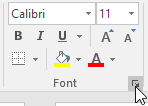
- Click the small arrow in the lower-right corner of the Alignment group on the Home tab.
- A dialog box will appear. Locate and select the Horizontal drop-down menu, select Center Across Selection, then click OK.
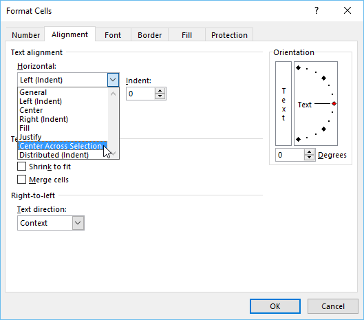
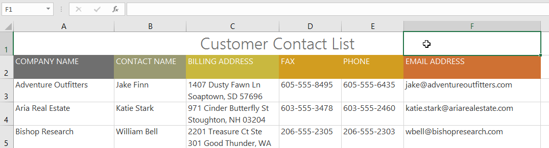
- The content will be centered across the selected cell range. As you can see, this creates the same visual result as merging and centering, but it preserves each cell within A1:F1.
Challenge!
- Open our practice workbook.
- Autofit Column Width for the entire workbook.
- Modify the row height for rows 3 to 14 to 22.5 (30 pixels).
- Delete row 10.
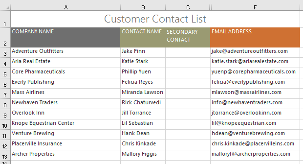
- Insert a column to the left of column C. Type SECONDARY CONTACT in cell C2.
- Make sure cell C2 is still selected and choose Wrap Text.
- Merge and Center cells A1:F1.
- Hide the Billing Address and Phone columns.
- When you're finished, your workbook should look something like this:
Lesson 7: Formatting Cells
Introduction
All cell content uses the same formatting by default, which can make it difficult to read a workbook with a lot of information. Basic formatting can customize the look and feel of your workbook, allowing you to draw attention to specific sections and making your content easier to view and understand.
Optional: Download our practice workbook.
Watch the video below to learn more about formatting cells in Excel.
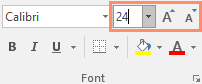
To change the font size:
- Select the cell(s) you want to modify.
- On the Home tab, click the drop-down arrow next to the Font Size command, then select the desired font size. In our example, we will choose 24 to make the text larger.
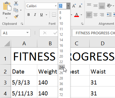
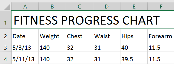
- The text will change to the selected font size.
You can also use the Increase Font Size and Decrease Font Size commands or enter a custom font size using your keyboard.
To change the font:
By default, the font of each new workbook is set to Calibri. However, Excel provides many other fonts you can use to customize your cell text. In the example below, we'll format our title cell to help distinguish it from the rest of the worksheet.
- Select the cell(s) you want to modify.
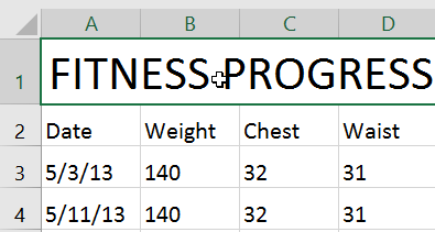
- On the Home tab, click the drop-down arrow next to the Font command, then select the desired font. In our example, we'll choose Century Gothic.
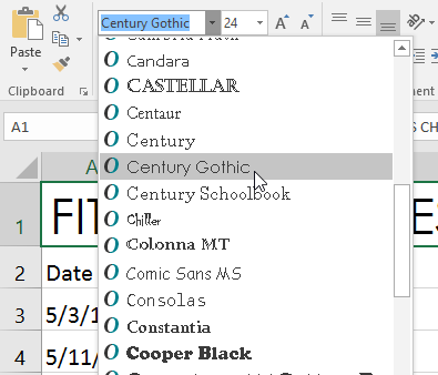
- The text will change to the selected font.
When creating a workbook in the workplace, you'll want to select a font that is easy to read. Along with Calibri, standard reading fonts include Cambria, Times New Roman, and Arial.
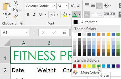
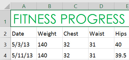
To change the font color:
- Select the cell(s) you want to modify.
- On the Home tab, click the drop-down arrow next to the Font Color command, then select the desired font color. In our example, we'll choose Green.
- The text will change to the selected font color.
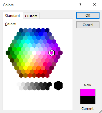
Select More Colors at the bottom of the menu to access additional color options. We've changed the font color to a bright pink.
To use the Bold, Italic, and Underline commands:
- Select the cell(s) you want to modify.
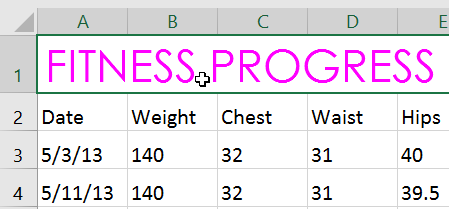
- Click the Bold (B), Italic (I), or Underline (U) command on the Home tab. In our example, we'll make the selected cells bold.
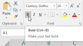
- The selected style will be applied to the text.
You can also press Ctrl+B on your keyboard to make selected text bold, Ctrl+I to apply italics, and Ctrl+U to apply an underline.
Cell borders and fill colors
Cell borders and fill colors allow you to create clear and defined boundaries for different sections of your worksheet. Below, we'll add cell borders and fill color to our header cells to help distinguish them from the rest of the worksheet.
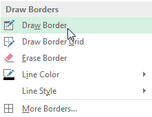
To add a fill color:
- Select the cell(s) you want to modify.
- On the Home tab, click the drop-down arrow next to the Fill Color command, then select the fill color you want to use. In our example, we'll choose a dark gray.
- The selected fill color will appear in the selected cells. We've also changed the font color to white to make it more readable with this dark fill color.
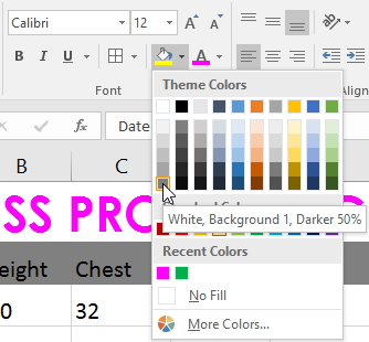
To add a border:
- Select the cell(s) you want to modify.
- On the Home tab, click the drop-down arrow next to the Borders command, then select the border style you want to use. In our example, we'll choose to display All Borders.
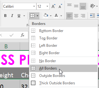
- The selected border style will appear.
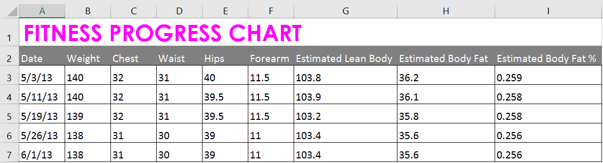
You can draw borders and change the line style and color of borders with the Draw Borders tools at the bottom of the Borders drop-down menu.
Cell styles
Instead of formatting cells manually, you can use Excel's predesigned cell styles. Cell styles are a quick way to include professional formatting for different parts of your workbook, such as titles and headers.
To apply a cell style:
In our example, we'll apply a new cell style to our existing title and header cells.
- Select the cell(s) you want to modify.
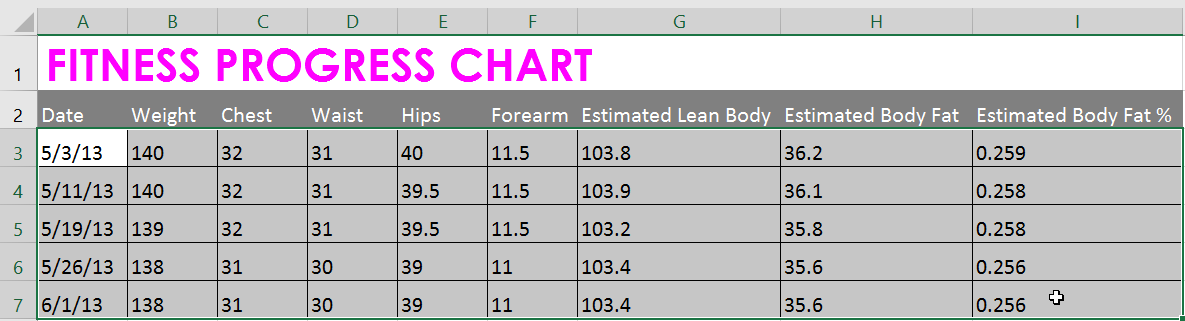
- Click the Cell Styles command on the Home tab, then choose the desired style from the drop-down menu.
- The selected cell style will appear.
Applying a cell style will replace any existing cell formatting except for text alignment. You may not want to use cell styles if you've already added a lot of formatting to your workbook.
Text alignment
By default, any text entered into your worksheet will be aligned to the bottom-left of a cell, while any numbers will be aligned to the bottom-right. Changing the alignment of your cell content allows you to choose how the content is displayed in any cell, which can make your cell content easier to read.
Left Align: Aligns content to the left border of the cell
Center Align: Aligns content an equal distance from the left and right borders of the cell
Right Align: Aligns content to the right border of the cell
Top Align: Aligns content to the top border of the cell
Middle Align: Aligns content an equal distance from the top and bottom borders of the cell
Bottom Align: Aligns content to the bottom border of the cell
To change horizontal text alignment:
In our example below, we'll modify the alignment of our title cell to create a more polished look and further distinguish it from the rest of the worksheet.
- Select the cell(s) you want to modify.
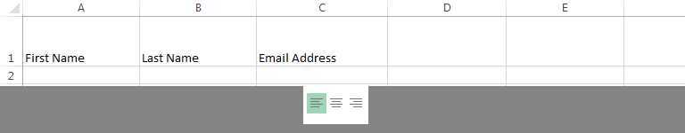
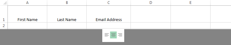
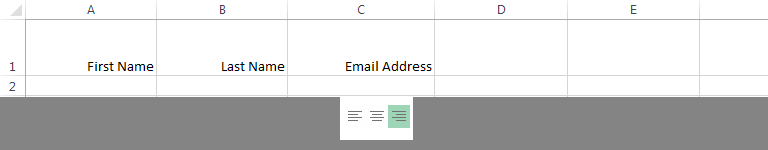
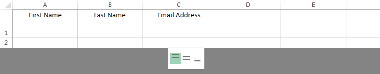
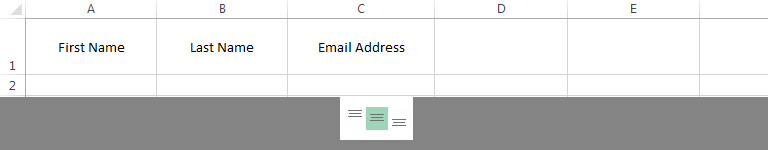
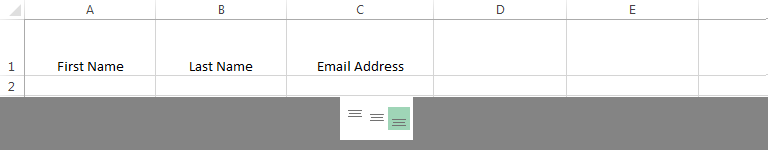
- Select one of the three horizontal alignment commands on the Home tab. In our example, we'll choose Center Align.
- The text will realign.
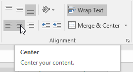
To change vertical text alignment:
- Select the cell(s) you want to modify.
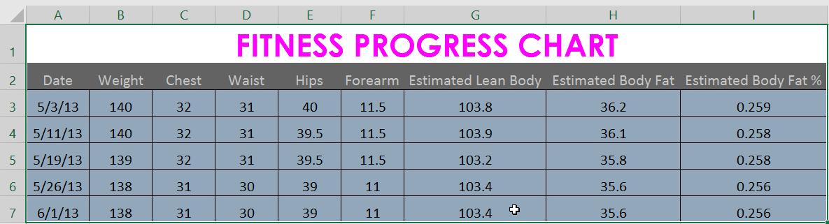
- Select one of the three vertical alignment commands on the Home tab. In our example, we'll choose Middle Align.
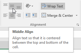
- The text will realign.
You can apply both vertical and horizontal alignment settings to any cell.
Format Painter
If you want to copy formatting from one cell to another, you can use the Format Painter command on the Home tab. When you click the Format Painter, it will copy all of the formatting from the selected cell. You can then click and drag over any cells you want to paste the formatting to.
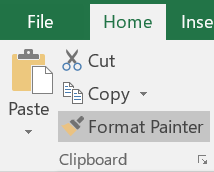
Watch the video below to learn two different ways to use the Format Painter.
Challenge!
- Open our practice workbook.
- Click the Challenge worksheet tab in the bottom-left of the workbook.
- Change the cell style in cells A2:H2 to Accent 3.
- Change the font size of row 1 to 36 and the font size for the rest of the rows to 18.
- Bold and underline the text in row 2.
- Change the font of row 1 to a font of your choice.
- Change the font of the rest of the rows to a different font of your choice.
- Change the font color of row 1 to a color of your choice.
- Select all of the text in the worksheet, and change the horizontal alignment to center align and the vertical alignment to middle align.
- When you're finished, your worksheet should look something like this:
Lesson 8: Understanding Number Formats
What are number formats?
Whenever you're working with a spreadsheet, it's a good idea to use appropriate number formats for your data. Number formats tell your spreadsheet exactly what type of data you're using, like percentages (%), currency ($), times, dates, and so on.
Watch the video below to learn more about number formats in Excel.
Why use number formats?
Number formats don't just make your spreadsheet easier to read—they also make it easier to use. When you apply a number format, you're telling your spreadsheet exactly what types of values are stored in a cell. For example, the date format tells the spreadsheet that you're entering specific calendar dates. This allows the spreadsheet to better understand your data, which can help ensure that your data remains consistent and that your formulas are calculated correctly.
If you don't need to use a specific number format, the spreadsheet will usually apply the general number format by default. However, the general format may apply some small formatting changes to your data.
Applying number formats
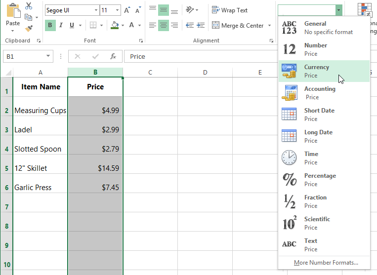
Just like other types of formatting, such as changing the font color, you'll apply number formats by selecting cells and choosing the desired formatting option. There are two main ways to choose a number format:
- Go to the Home tab, click the Number Format drop-down menu in the Number group, and select the desired format.
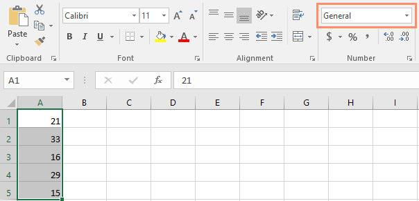
- You can also click one of the quick number-formatting commands below the drop-down menu.
You can also select the desired cells and press Ctrl+1 on your keyboard to access more number-formatting options.
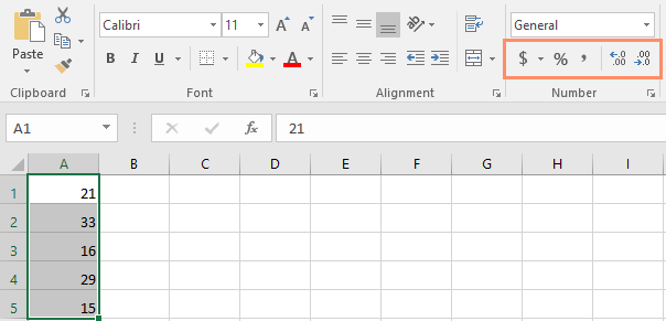
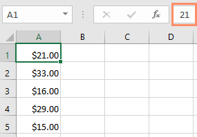
In this example, we've applied the Currency number format, which adds currency symbols ($) and displays two decimal places for any numerical values.
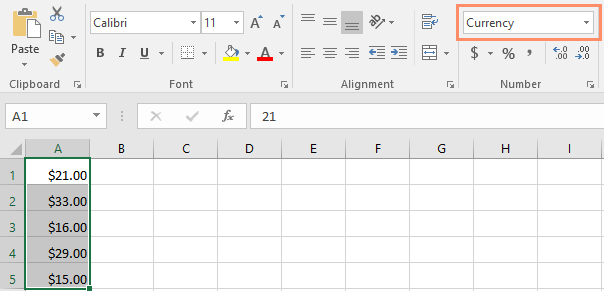
If you select any cells with number formatting, you can see the actual value of the cell in the formula bar. The spreadsheet will use this value for formulas and other calculations.
Using number formats correctly
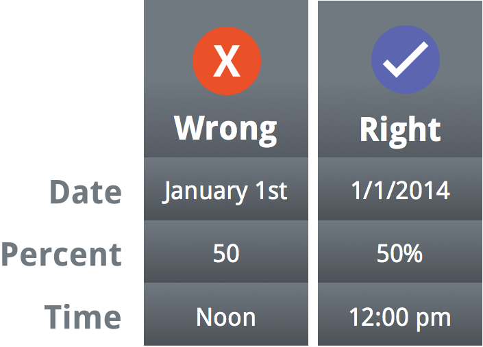
There's more to number formatting than selecting cells and applying a format. Spreadsheets can actually apply a lot of number formatting automatically based on the way you enter data. This means you'll need to enter data in a way the program can understand, and then ensure that those cells are using the proper number format. For example, the image below shows how to use number formats correctly for dates, percentages, and times:
Now that you know more about how number formats work, we'll look at a few different number formats in action.
Percentage formats
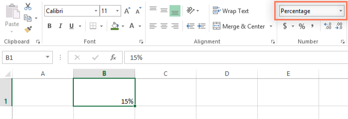
One of the most helpful number formats is the percentage (%) format. It displays values as percentages, such as 20% or 55%. This is especially helpful when calculating things like the cost of sales tax or a tip. When you type a percent sign (%) after a number, the percentage number format will be be applied to that cell automatically.
As you may remember from math class, a percentage can also be written as a decimal. So 15% is the same thing as 0.15, 7.5% is 0.075, 20% is 0.20, 55% is 0.55, and so on. You can review this lesson from our Math tutorials to learn more about converting percentages to decimals.
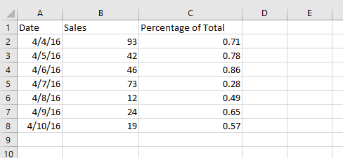
There are many times when percentage formatting will be useful. For example, in the images below, notice how the sales tax rate is formatted differently for each spreadsheet (5, 5%, and 0.05):
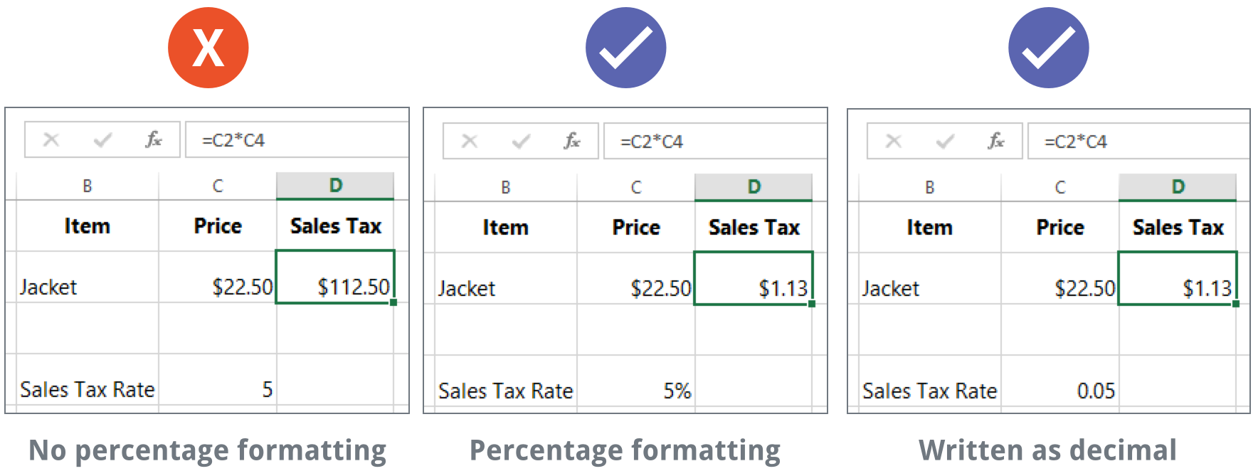
As you can see, the calculation in the spreadsheet on the left didn't work correctly. Without the percentage number format, our spreadsheet thinks we want to multiply $22.50 by 5, not 5%. And while the spreadsheet on the right still works without percentage formatting, the spreadsheet in the middle is easier to read.
Date formats
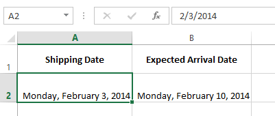
Whenever you're working with dates, you'll want to use a date format to tell the spreadsheet that you're referring to specific calendar dates, such as July 15, 2014. Date formats also allow you to work with a powerful set of date functions that use time and date information to calculate an answer.
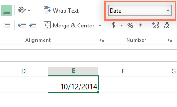
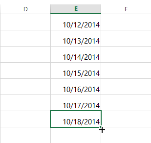
Spreadsheets don't understand information the same way a person would. For instance, if you type October into a cell, the spreadsheet won't know you're entering a date so it will treat it like any other text. Instead, when you enter a date, you'll need to use a specific format your spreadsheet understands, such as month/day/year (or day/month/year depending on which country you're in). In the example below, we'll type 10/12/2014 for October 12, 2014. Our spreadsheet will then automatically apply the date number format for the cell.
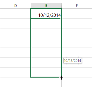
Now that we have our date correctly formatted, we can do many different things with this data. For example, we could use the fill handle to continue the dates through the column, so a different day appears in each cell:
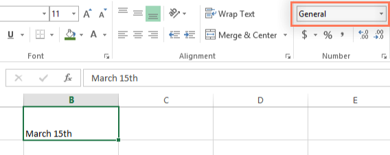
If the date formatting isn't applied automatically, it means the spreadsheet did not understand the data you entered. In the example below, we've typed March 15th. The spreadsheet did not understand that we were referring to a date, so this cell is still using the general number format.
On the other hand, if we type March 15 (without the "th"), the spreadsheet will recognize it as a date. Because it doesn't include a year, the spreadsheet will automatically add the current year so the date will have all of the necessary information. We could also type the date several other ways, such as 3/15, 3/15/2014, or March 15 2014, and the spreadsheet would still recognize it as a date.
Try entering the dates below into a spreadsheet and see if the date format is applied automatically:
- 10/12
- October
- October 12
- October 2016
- 10/12/2016
- October 12, 2016
- 2016
- October 12th
If you want to add the current date to a cell, you can use the Ctrl+; shortcut, as shown in the video below.
Other date formatting options
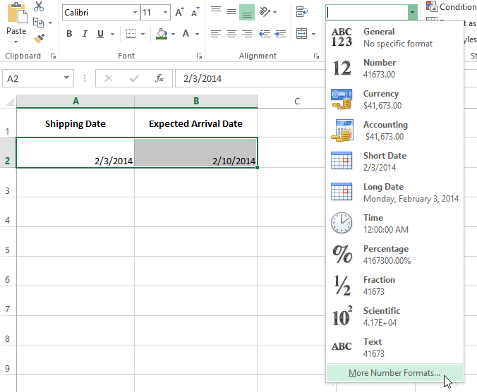
To access other date formatting options, select the Number Format drop-down menu and choose More Number Formats. These are options to display the date differently, like including the day of the week or omitting the year.
The Format Cells dialog box will appear. From here, you can choose the desired date formatting option.
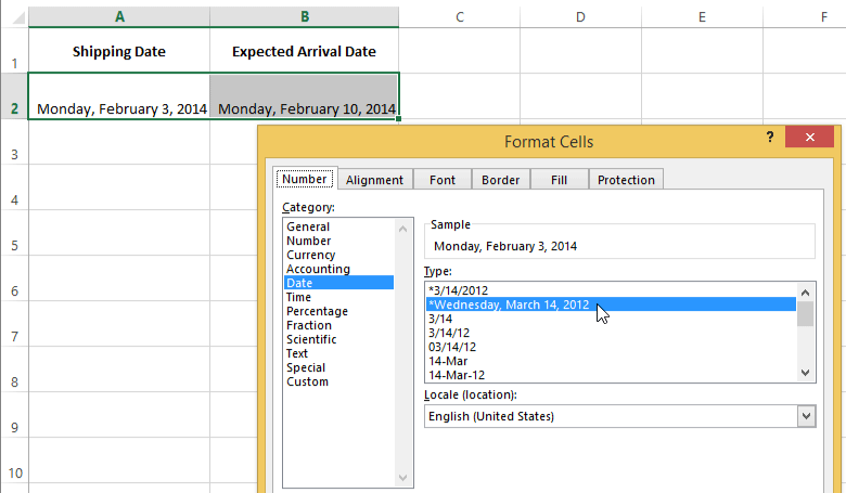
As you can see in the formula bar, a custom date format doesn't change the actual date in our cell—it just changes the way it's displayed.
Number formatting tips
Here are a few tips for getting the best results with number formatting:
- Apply number formatting to an entire column: If you're planning to use one column for a certain type of data, like dates or percentages, you may find it easiest to select the entire column by clicking the column letter and applying the desired number formatting. This way, any data you add to this column in the future will already have the correct number format. Note that the header row usually won't be affected by number formatting.
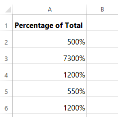
- Double-check your values after applying number formatting: If you apply number formatting to existing data, you may have unexpected results. For example, applying percentage (%) formatting to a cell with a value of 5 will give you 500%, not 5%. In this case, you'd need to retype the values correctly in each cell.
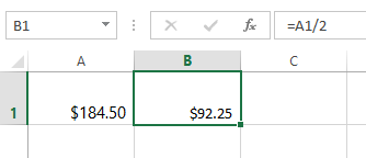
- If you reference a cell with number formatting in a formula, the spreadsheet may automatically apply the same number formatting to the new cell. For example, if you use a value with currency formatting in a formula, the calculated value will also use the currency number format.
- If you want your data to appear exactly as entered, you'll need to use the text number format. This format is especially good for numbers you don't want to perform calculations with, such as phone numbers, zip codes, or numbers that begin with 0, like 02415. For best results, you may want to apply the text number format before entering data into these cells.
Increase and Decrease Decimal
The Increase Decimal and Decrease Decimal commands allow you to control how many decimal places are displayed in a cell. These commands don't change the value of the cell; instead, they display the value to a set number of decimal places.
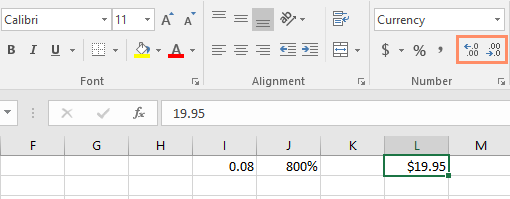
Decreasing the decimal will display the value rounded to that decimal place, but the actual value in the cell will still be displayed in the formula bar.
The Increase/Decrease Decimal commands don't work with some number formats, like Date and Fraction.
Challenge!
- Open our practice workbook.
- In cell D2, type today's date and press Enter.
- Click cell D2 and verify that it is using a Date number format. Try changing it to a different date format (for example, Long Date).
- In cell D2, use the Format Cells dialog box to choose the 14-Mar-12 date format.
- Change the sales tax rate in cell D8 to the Percentage format.
- Apply the Currency format to all of column B.
- In cell D8, use the Increase Decimal or Decrease Decimal command to change the number of decimal places to one. It should now display 7.5%.
- When you're finished, your spreadsheet should look like this:
Lesson 9: Working with Multiple Worksheets
Introduction
Every workbook contains at least one worksheet by default. When working with a large amount of data, you can create multiple worksheets to help organize your workbook and make it easier to find content. You can also group worksheets to quickly add information to multiple worksheets at the same time.
Optional: Download our practice workbook.
Watch the video below to learn more about using multiple worksheets.
To insert a new worksheet:
- Locate and select the New sheet button near the bottom-right corner of the Excel window.
- A new blank worksheet will appear.
By default, any new workbook you create in Excel will contain one worksheet, called Sheet1. To change the default number of worksheets, navigate to Backstage view, click Options, then choose the desired number of worksheets to include in each new workbook.
To copy a worksheet:
If you need to duplicate the content of one worksheet to another, Excel allows you to copy an existing worksheet.
- Right-click the worksheet you want to copy, then select Move or Copy from the worksheet menu.
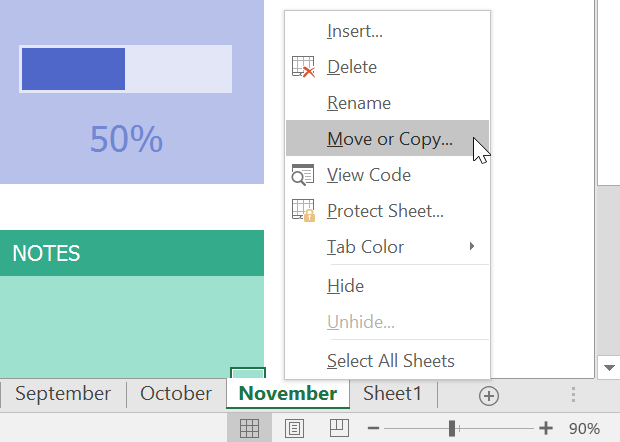
- The Move or Copy dialog box will appear. Choose where the sheet will appear in the Before sheet: field. In our example, we'll choose (move to end) to place the worksheet to the right of the existing worksheet.
- Check the box next to Create a copy, then click OK.

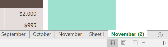
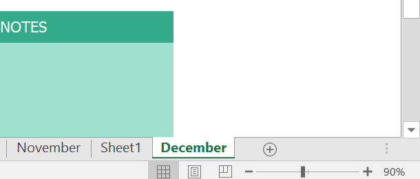
- The worksheet will be copied. It will have the same title as the original worksheet, as well as a version number. In our example, we copied the November worksheet, so our new worksheet is named November (2). All content from the November worksheet has also been copied to the new worksheet.
You can also copy a worksheet to an entirely different workbook. You can select any workbook that is currently open from the To book: drop-down menu.
To rename a worksheet:
- Right-click the worksheet you want to rename, then select Rename from the worksheet menu.
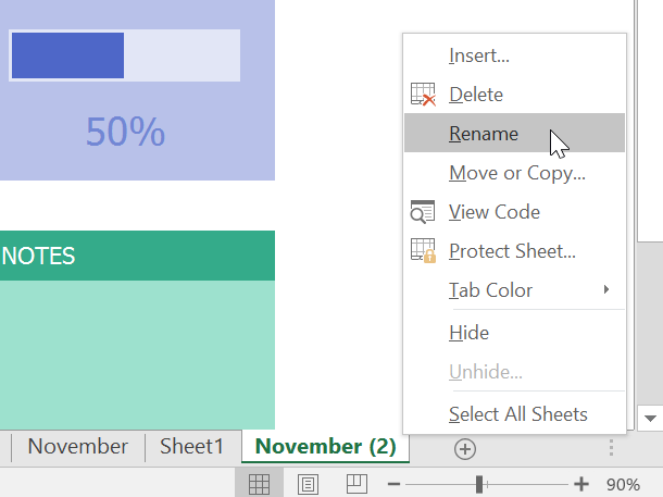
- Type the desired name for the worksheet.
- Click anywhere outside the worksheet tab, or press Enter on your keyboard. The worksheet will be renamed.
To move a worksheet:
- Click and drag the worksheet you want to move until a small black arrow appears above the desired location.
- Release the mouse. The worksheet will be moved.
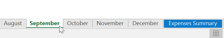
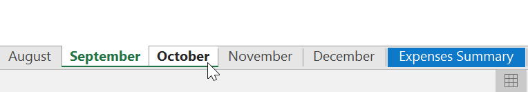
To change the worksheet tab color:
- Right-click the desired worksheet tab, and hover the mouse over Tab Color. The Color menu will appear.
- Select the desired color.
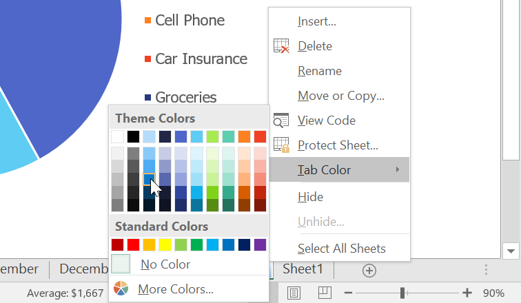
- The worksheet tab color will be changed.
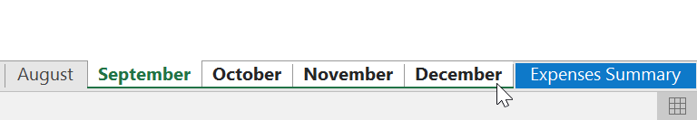
The worksheet tab color is considerably less noticeable when the worksheet is selected. Select another worksheet to see how the color will appear when the worksheet is not selected.
To delete a worksheet:
- Right-click the worksheet you want to delete, then select Delete from the worksheet menu.
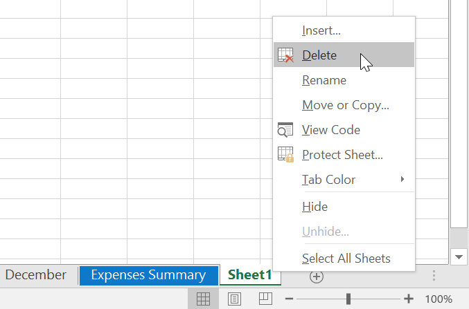
- The worksheet will be deleted from your workbook.
If you want to prevent specific worksheets from being edited or deleted, you can protect them by right-clicking the desired worksheet and selecting Protect Sheet from the worksheet menu.
Switching between worksheets
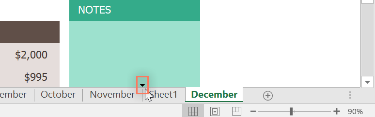
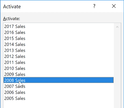
If you want to view a different worksheet, you can simply click the tab to switch to that worksheet. However, with larger workbooks this can sometimes become tedious, as it may require scrolling through all of the tabs to find the one you want. Instead, you can simply right-click the scroll arrows in the lower-left corner, as shown below.
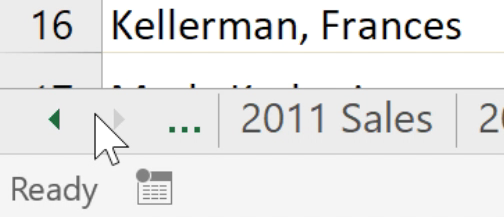
A dialog box will appear with a list of all of the sheets in your workbook. You can then double-click the sheet you want to jump to.
Watch the video below to see this shortcut in action.
Grouping and ungrouping worksheets
You can work with each worksheet individually, or you can work with multiple worksheets at the same time. Worksheets can be combined together into a group. Any changes made to one worksheet in a group will be made to every worksheet in the group.
To group worksheets:
- Select the first worksheet you want to include in the worksheet group.
- Press and hold the Ctrl key on your keyboard. Select the next worksheet you want in the group.
- Continue to select worksheets until all of the worksheets you want to group are selected, then release the Ctrl key. The worksheets are now grouped.
While worksheets are grouped, you can navigate to any worksheet within the group. Any changes made to one worksheet will appear on every worksheet in the group. However, if you select a worksheet that is not in the group, all of your worksheets will become ungrouped.
To ungroup worksheets:
- Right-click a worksheet in the group, then select Ungroup Sheets from the worksheet menu.
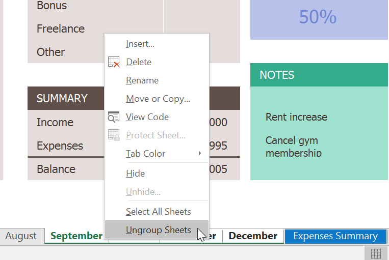
- The worksheets will be ungrouped. Alternatively, you can simply click any worksheet not included in the group to ungroup all worksheets.
Challenge!
- Open our practice workbook.
- Insert a new worksheet, and rename it Q1 Summary.
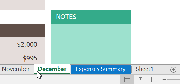
- Move the Expenses Summary worksheet to the far right, then move the Q1 Summary worksheet so that it is between March and April.
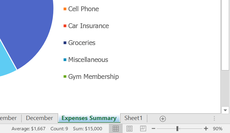
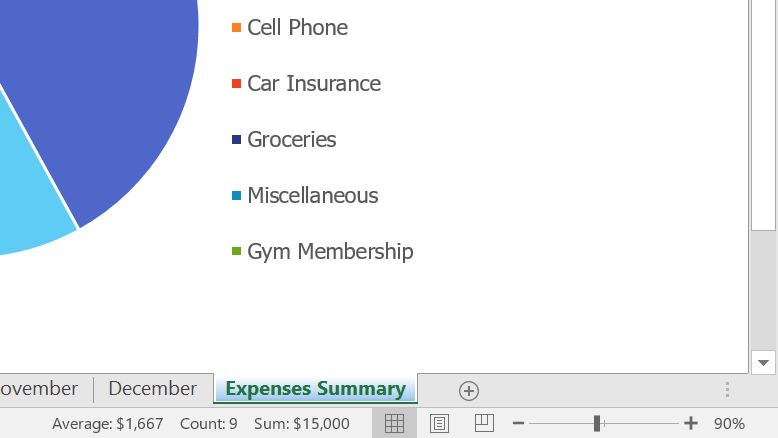
- Create a copy of the Expenses Summary worksheet by right-clicking the tab. Do not just copy and paste the content of the worksheet into a new worksheet.
- Change the color of the January tab to blue and the color of the February tab to red.
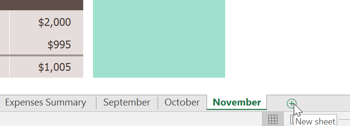
- Group the worksheets September, October, and November.
- When you're finished, your workbook should look something like this:
Lesson 10: Using Find & Replace
Introduction
When working with a lot of data in Excel, it can be difficult and time consuming to locate specific information. You can easily search your workbook using the Find feature, which also allows you to modify content using the Replace feature.
Optional: Download our practice workbook.
Watch the video below to learn more about using Find & Replace.
To find content:
In our example, we'll use the Find command to locate a specific department in this list.
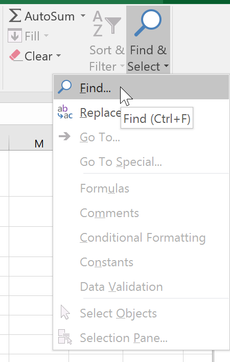
- From the Home tab, click the Find and Select command, then select Find from the drop-down menu.
- The Find and Replace dialog box will appear. Enter the content you want to find. In our example, we'll type the department's name.
- Click Find Next. If the content is found, the cell containing that content will be selected.
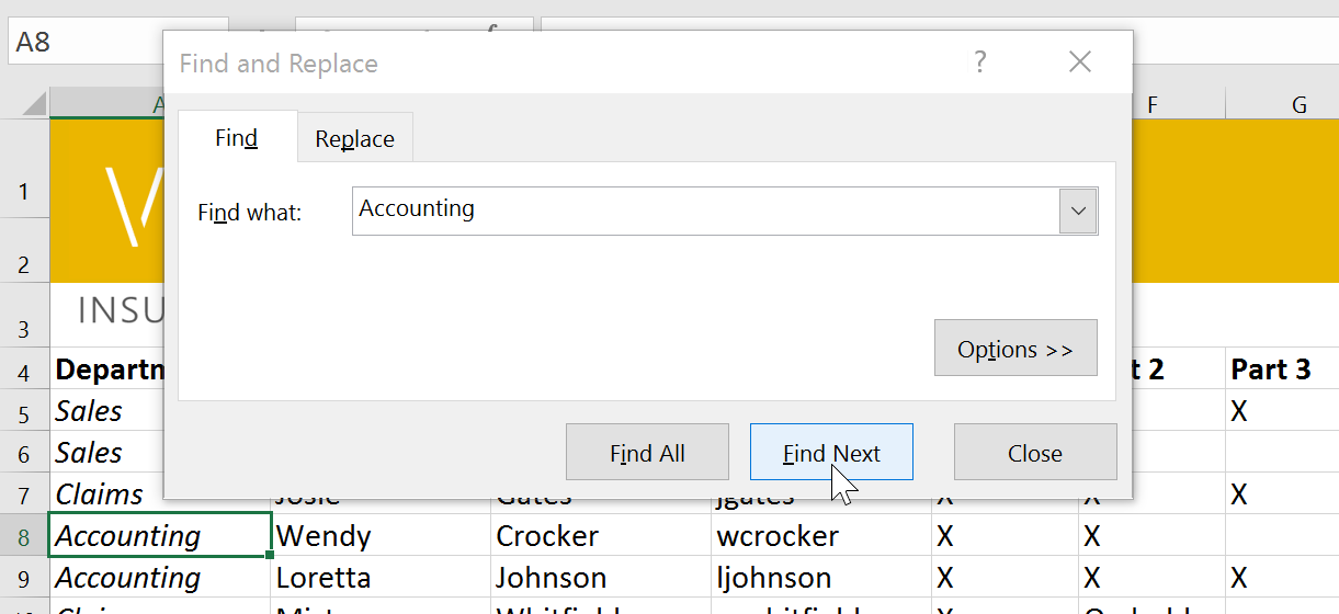
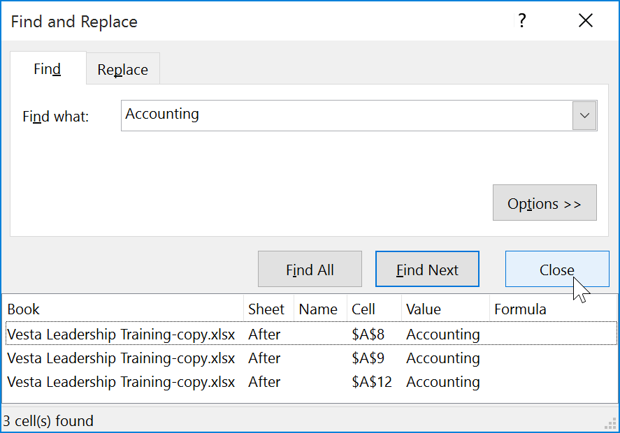
- Click Find Next to find further instances or Find All to see every instance of the search term.
- When you are finished, click Close to exit the Find and Replace dialog box.
You can also access the Find command by pressing Ctrl+F on your keyboard.
Click Options to see advanced search criteria in the Find and Replace dialog box.

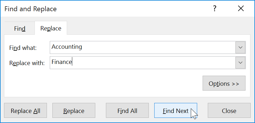
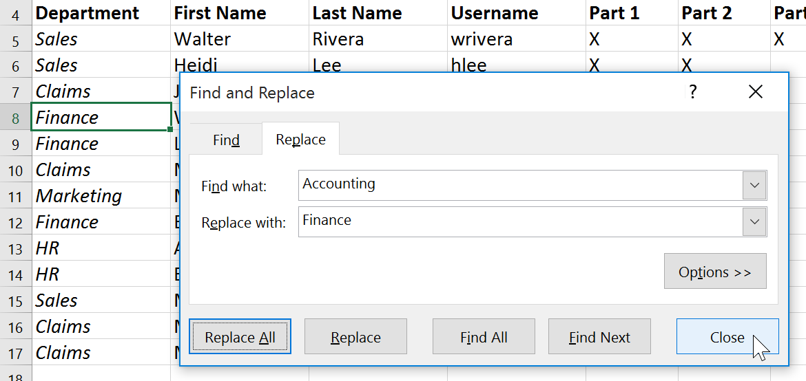
To replace cell content:
At times, you may discover that you've repeatedly made a mistake throughout your workbook (such as misspelling someone's name) or that you need to exchange a particular word or phrase for another. You can use Excel's Find and Replace feature to make quick revisions. In our example, we'll use Find and Replace to correct a list of department names.
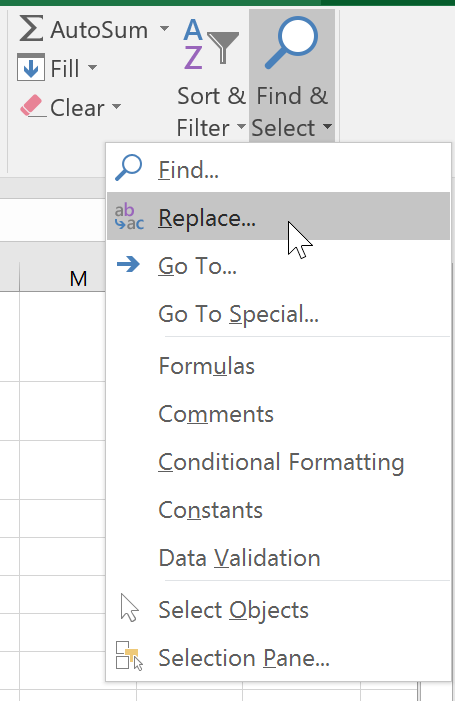
- From the Home tab, click the Find and Select command, then select Replace from the drop-down menu.
- The Find and Replace dialog box will appear. Type the text you want to find in the Find what: field.
- Type the text you want to replace it with in the Replace with: field, then click Find Next.
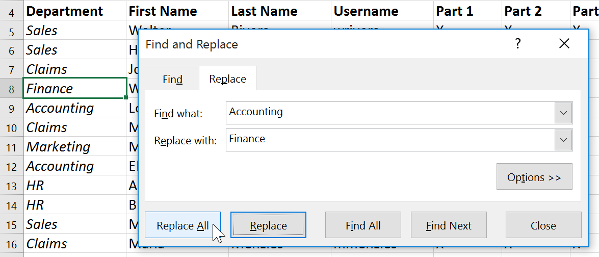
- If the content is found, the cell containing that content will be selected.
- Review the text to make sure you want to replace it.
- If you want to replace it, select one of the replace options. Choosing Replace will replace individual instances, while Replace All will replace every instance of the text throughout the workbook. In our example, we'll choose this option to save time.
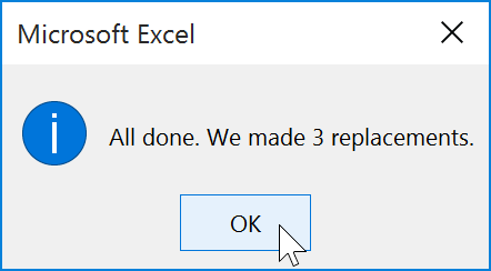
A dialog box will appear, confirming the number of replacements made. Click OK to continue.
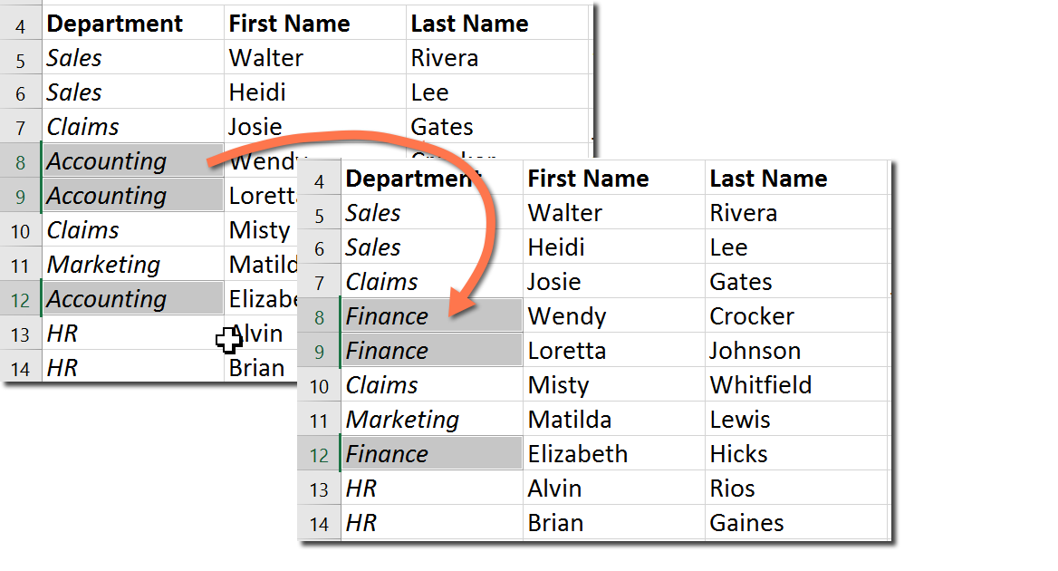
The selected cell content will be replaced.
- When you are finished, click Close to exit the Find and Replace dialog box.
Generally, it's best to avoid using Replace All because it doesn't give you the option of skipping anything you don't want to change. You should only use this option if you're absolutely sure it won't replace anything you didn't intend it to.
Challenge!
- Open our practice workbook.
- Click the Challenge tab in the bottom-left of the workbook.
- Crystal Lewis was married and changed her last name to Taylor. Use Find and Replace to change Crystal's last name from Lewis to Taylor. Be careful to only change Crystal's last name!
- Find and replace Bio with Biology. Be careful not to change the major Biomedical Engineering!
- Use Find and Replace All to replace the Physics major to Physical Science.
- When you're finished, your worksheet should look like this:

Lesson 11: Checking Spelling
Introduction
Before sharing a workbook, you'll want to make sure it doesn't include any spelling errors. Fortunately, Excel includes a Spell Check tool you can use to make sure everything in your workbook is spelled correctly.
If you've used the Spell Check feature in Microsoft Word, just be aware that the Spell Check tool in Excel, while helpful, is not as powerful. For example, it won't check for grammar issues or check spelling as you type.
Optional: Download our practice workbook.
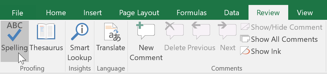
To use Spell Check:
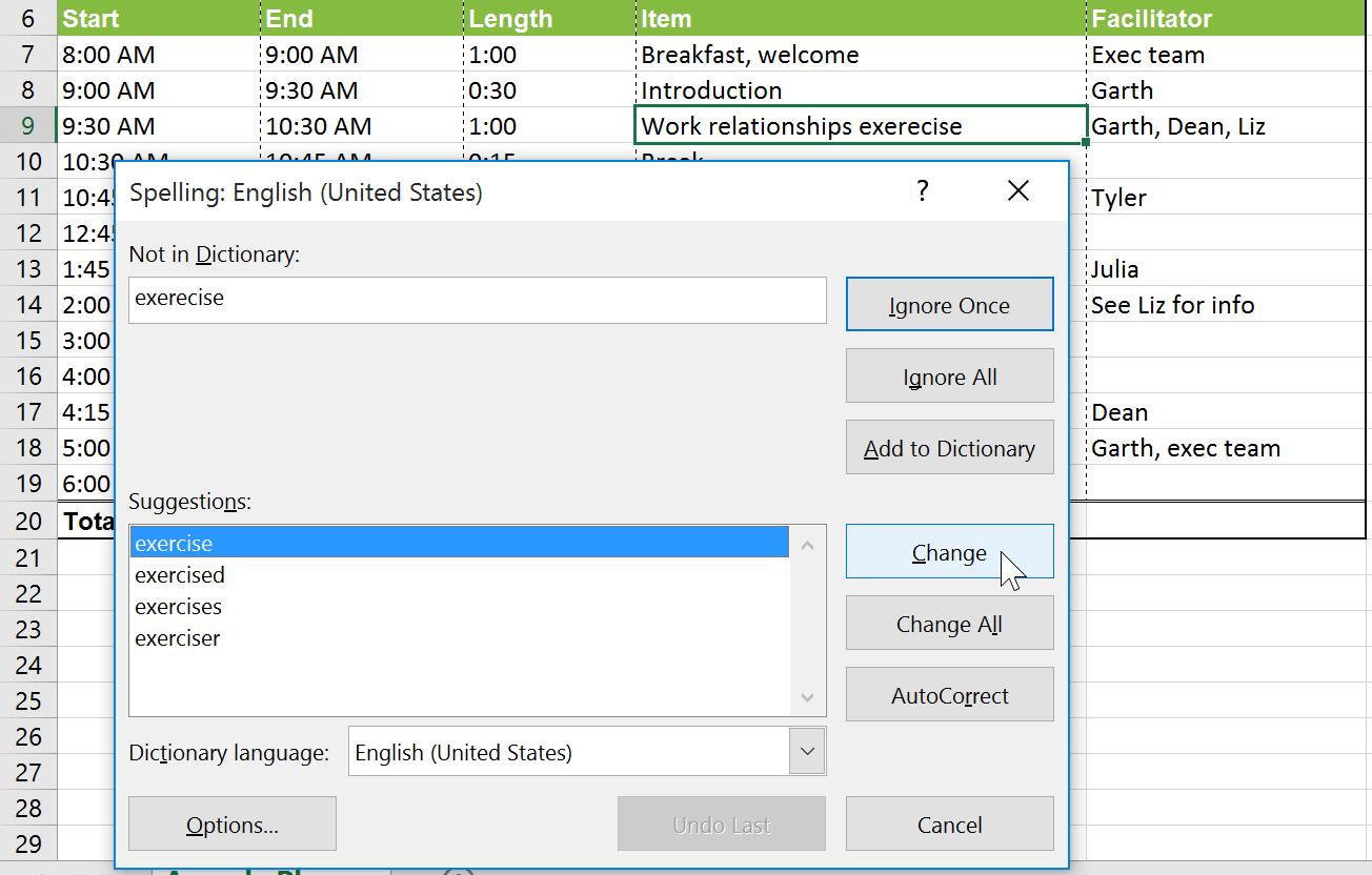
- From the Review tab, click the Spelling command.
- The Spelling dialog box will appear. For each spelling error in your worksheet, Spell Check will try to offer suggestions for the correct spelling. Choose a suggestion, then click Change to correct the error.
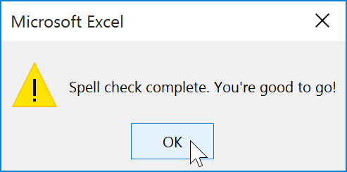
- A dialog box will appear after reviewing all spelling errors. Click OK to close Spell Check.
If there are no appropriate suggestions, you can also enter the correct spelling manually.
Ignoring spelling "errors"
Spell Check isn't always correct. It will sometimes mark certain words as incorrect even if they're spelled correctly. This often happens with names, which may not be in the dictionary. You can choose not to change a spelling "error" using one of the following three options:
- Ignore Once: This will skip the word without changing it.
- Ignore All: This will skip the word without changing it and also skip all other instances of the word in your worksheet.
- Add: This adds the word to the dictionary so it will never appear as an error again. Make sure the word is spelled correctly before choosing this option.
Challenge!
- Open our practice workbook.
- Click the Challenge worksheet tab in the bottom-left of the workbook.
- Run the Spell Check to correct any spelling errors in the workbook.
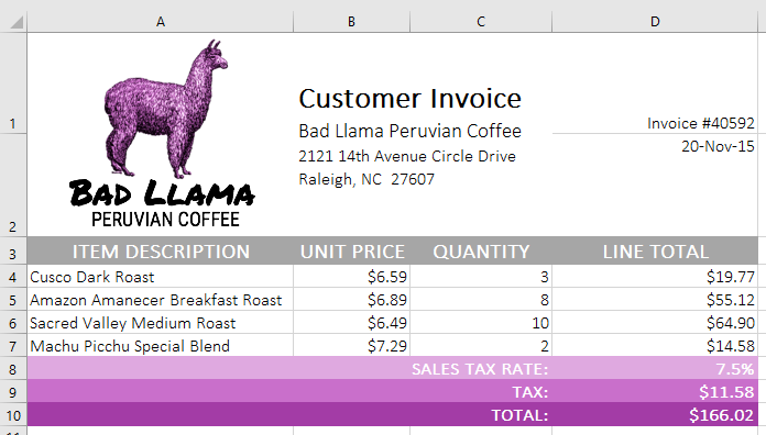
- Correct the words coffe and medum using the suggested spelling.
- Ignore the spelling suggestion for the word Amanecer.
- When you're finished, your worksheet should look like this:
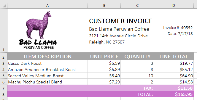
- Bonus Step! There is one error Spell Check didn't catch. Can you spot it? Hint: It's in one of the item descriptions.
Lesson 12: Page Layout and Printing
Introduction
There may be times when you want to print a workbook to view and share your data offline. Once you've chosen your page layout settings, it's easy to preview and print a workbook from Excel using the Print pane.
Optional: Download our practice workbook.
Watch the video below to learn more about page layout and printing.
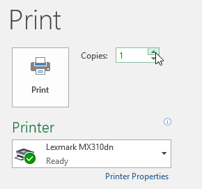
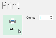
To access the Print pane:
- Select the File tab. Backstage view will appear.
- Select Print. The Print pane will appear.
Click the buttons in the interactive below to learn more about using the Print pane.
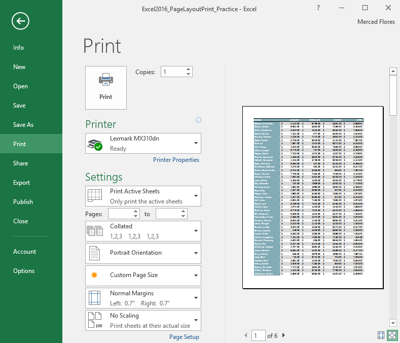
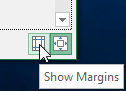
Show Margins / Zoom to Page
The Zoom to Page button on the right will zoom in and out in the Preview pane.
The Show Margins button on the left will show the margins in the Preview pane.
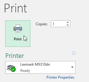
To print a workbook:
- Navigate to the Print pane, then select the desired printer.
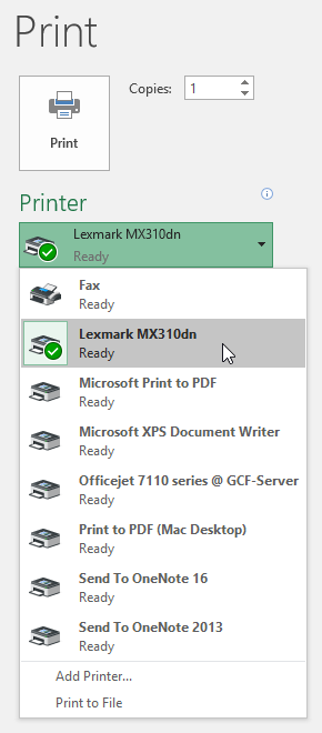
- Enter the number of copies you want to print.
- Select any additional settings if needed (see above interactive).
- Click Print.
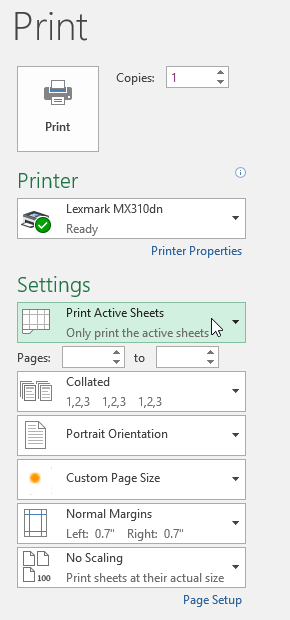
Choosing a print area
Before you print an Excel workbook, it's important to decide exactly what information you want to print. For example, if you have multiple worksheets in your workbook, you will need to decide if you want to print the entire workbook or only active worksheets. There may also be times when you want to print only a selection of content from your workbook.
To print active sheets:
Worksheets are considered active when selected.
- Select the worksheet you want to print. To print multiple worksheets, click the first worksheet, hold the Ctrl key on your keyboard, then click any other worksheets you want to select.

- Navigate to the Print pane.
- Select Print Active Sheets from the Print Range drop-down menu.
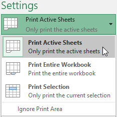
- Click the Print button.
To print the entire workbook:
- Navigate to the Print pane.
- Select Print Entire Workbook from the Print Range drop-down menu.
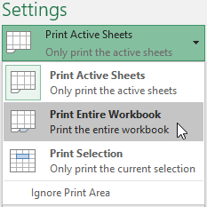
- Click the Print button.
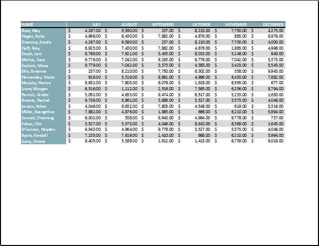
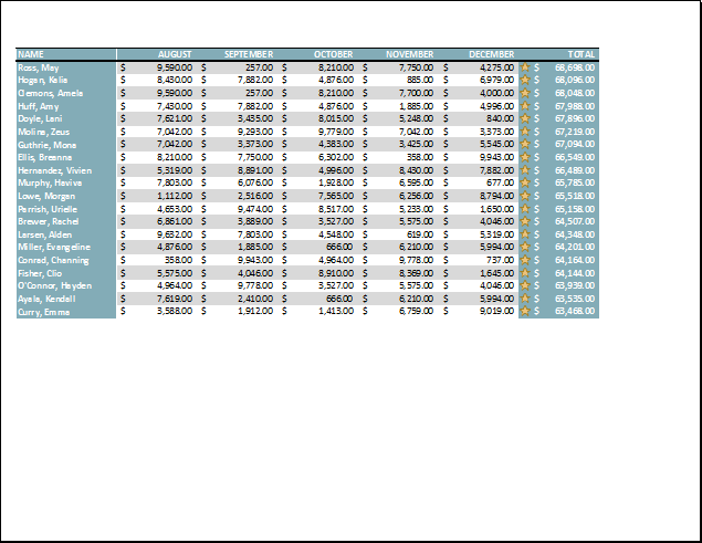
To print a selection:
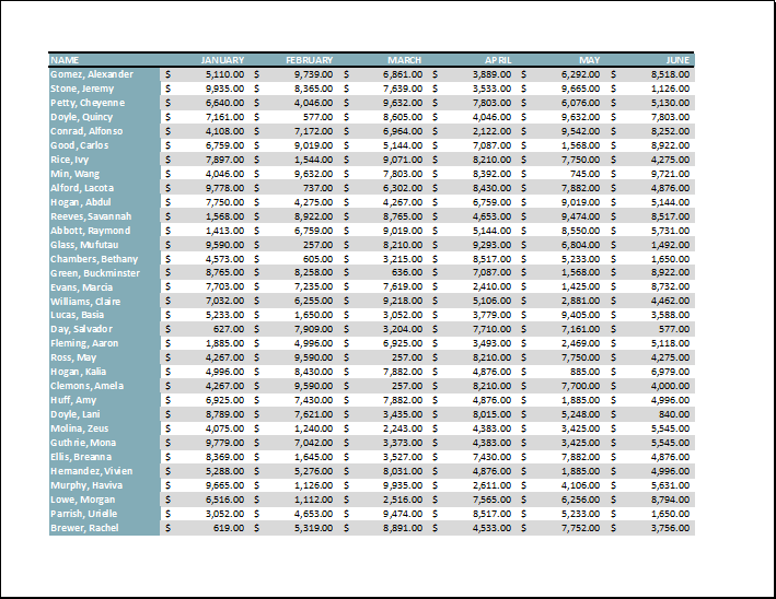
In our example, we'll print the records for the top 40 salespeople on the Central worksheet.
- Select the cells you want to print.
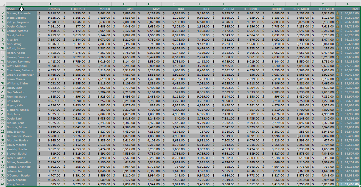
- Navigate to the Print pane.
- Select Print Selection from the Print Range drop-down menu.
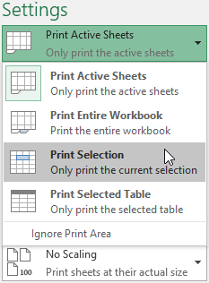
- A preview of your selection will appear in the Preview pane.
- Click the Print button to print the selection.
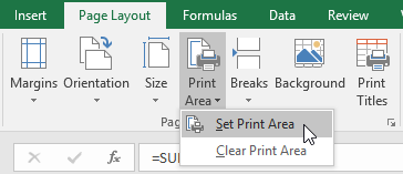
If you prefer, you can also set the print area in advance so you'll be able to visualize which cells will be printed as you work in Excel. Simply select the cells you want to print, click the Page Layout tab, select the Print Area command, then choose Set Print Area. Keep in mind that if you ever need to print the entire workbook, you'll need to clear the print area.
Adjusting content
On occasion, you may need to make small adjustments from the Print pane to fit your workbook content neatly onto a printed page. The Print pane includes several tools to help fit and scale your content, such as scaling and page margins.
To change page orientation:
Excel offers two page orientation options: landscape and portrait. Landscape orients the page horizontally, while portrait orients the page vertically. In our example, we'll set the page orientation to landscape.
- Navigate to the Print pane.
- Select the desired orientation from the Page Orientation drop-down menu. In our example, we'll select Landscape Orientation.
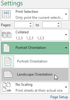
- The new page orientation will be displayed in the Preview pane.
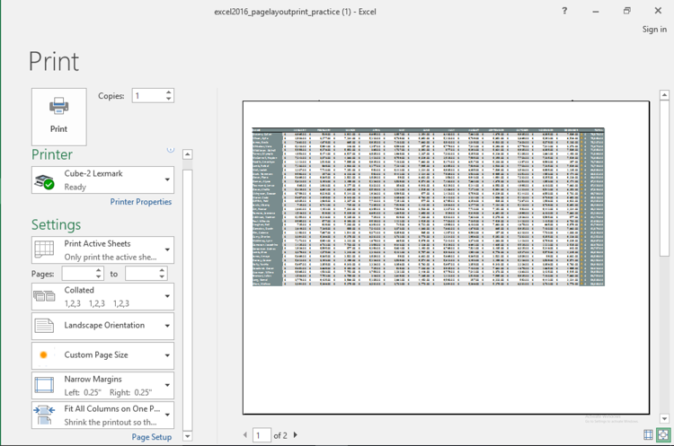
To fit content before printing:
If some of your content is being cut off by the printer, you can use scaling to fit your workbook to the page automatically.
- Navigate to the Print pane. In our example, we can see in the Preview pane that our content will be cut off when printed.
- Select the desired option from the Scaling drop-down menu. In our example, we'll select Fit All Columns on One Page.
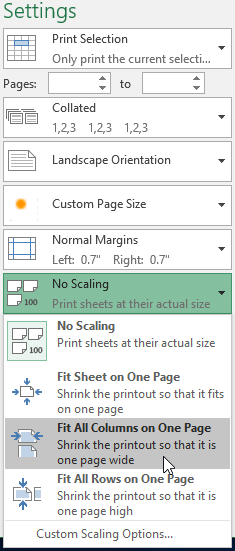
- The worksheet will be condensed to fit onto a single page.
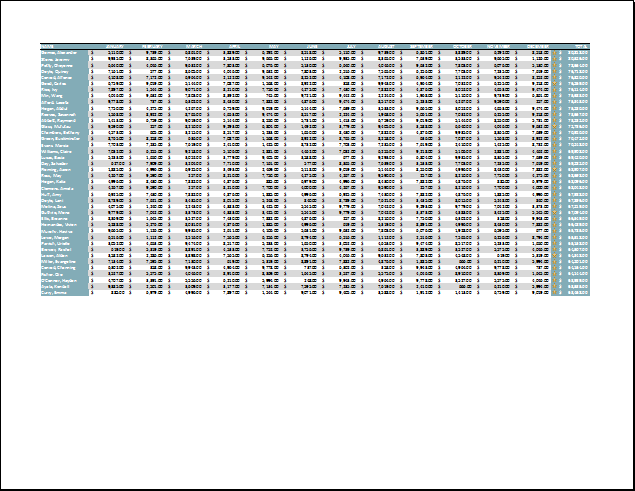
Keep in mind that worksheets will become more difficult to read as they are scaled down, so you may not want to use this option when printing a worksheet with a lot of information. In our example, we'll change the scaling setting back to No Scaling.
To include Print Titles:
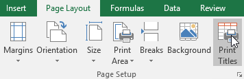
If your worksheet uses title headings, it's important to include these headings on each page of your printed worksheet. It would be difficult to read a printed workbook if the title headings appeared only on the first page. The Print Titles command allows you to select specific rows and columns to appear on each page.
- Click the Page Layout tab on the Ribbon, then select the Print Titles command.
- The Page Setup dialog box will appear. From here, you can choose rows or columns to repeat on each page. In our example, we'll repeat a row first.
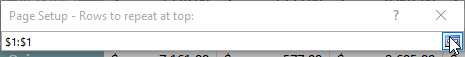
- Click the Collapse Dialog button next to the Rows to repeat at top: field.
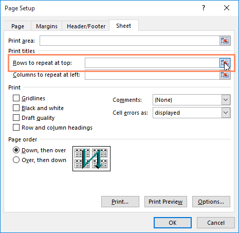
- The cursor will become a small selection arrow, and the Page Setup dialog box will be collapsed. Select the row(s) you want to repeat at the top of each printed page. In our example, we'll select row 1.
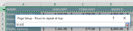
- Row 1 will be added to the Rows to repeat at top: field. Click the Collapse Dialog button again.
- The Page Setup dialog box will expand. To repeat a column as well, use the same process shown in steps 4 and 5. In our example, we've selected to repeat row 1 and column A.
- When you're satisfied with your selections, click OK.
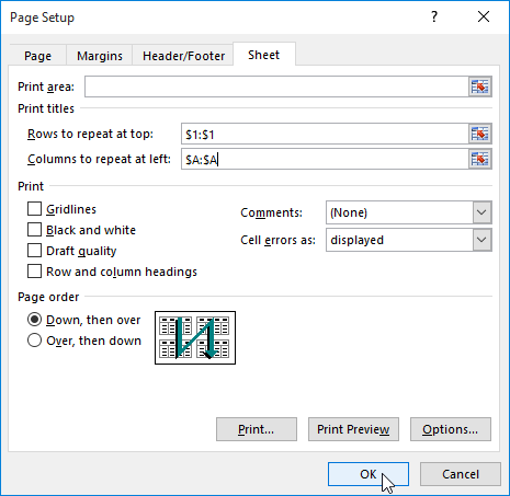
- In our example, row 1 appears at the top of every page, and column A appears at the left of every page.
To adjust page breaks:
- Click the Page Break Preview command to change to Page Break view.
- Vertical and horizontal blue dotted lines denote the page breaks. Click and drag one of these lines to adjust that page break.
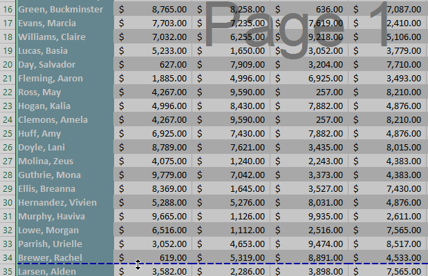
- In our example, we've set the horizontal page break between rows 21 and 22.
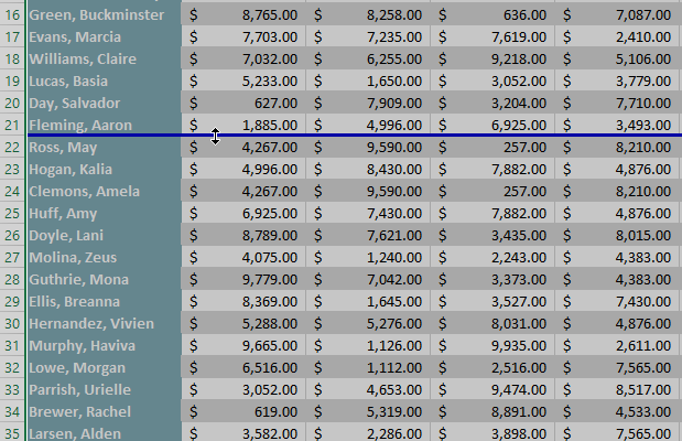
- In our example, all the pages now show the same number of rows due to the change in the page break.
To modify margins in the Preview pane:
A margin is the space between your content and the edge of the page. Sometimes you may need to adjust the margins to make your data fit more comfortably. You can modify page margins from the Print pane.
- Navigate to the Print pane.
- Select the desired margin size from the Page Margins drop-down menu. In our example, we'll select Narrow Margins.
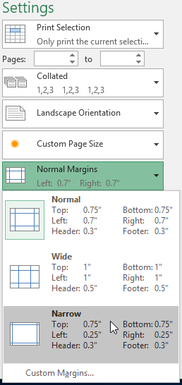
- The new page margins will be displayed in the Preview pane.
You can adjust the margins manually by clicking the Show Margins button in the lower-right corner, then dragging the margin markers in the Preview pane.
Challenge!
- Open our practice workbook.
- Click the East Coast tab at the bottom of the workbook.
- In the Page Layout tab, use the Print Titles feature to repeat row 1 at the top and column A at the left.
- Using the Page Break Preview command, move the break between rows 47 and 48 up so it's between rows 40 and 41.
- In Backstage view, open the Print Pane.
- In the Print pane, change the orientation to Landscape.
- Change the margins to Narrow.
- Change the scaling to Fit All Columns on One Page.
- When you are finished, your print preview should look like this:
Lesson 13: Intro to Formulas
Introduction
One of the most powerful features in Excel is the ability to calculate numerical information using formulas. Just like a calculator, Excel can add, subtract, multiply, and divide. In this lesson, we'll show you how to use cell references to create simple formulas.
Optional: Download our practice workbook.
Watch the video below to learn more about creating formulas in Excel.
Mathematical operators
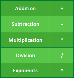
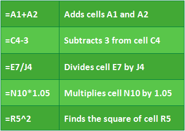
Excel uses standard operators for formulas, such as a plus sign for addition (+), a minus sign for subtraction (-), an asterisk for multiplication (*), a forward slash for division (/), and a caret (^) for exponents.
All formulas in Excel must begin with an equals sign (=). This is because the cell contains, or is equal to, the formula and the value it calculates.
Understanding cell references
While you can create simple formulas in Excel using numbers (for example, =2+2 or =5*5), most of the time you will use cell addresses to create a formula. This is known as making a cell reference. Using cell references will ensure that your formulas are always accurate because you can change the value of referenced cells without having to rewrite the formula.
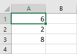
In the formula below, cell A3 adds the values of cells A1 and A2 by making cell references:
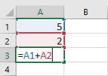
When you press Enter, the formula calculates and displays the answer in cell A3:
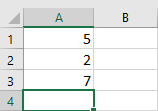
If the values in the referenced cells change, the formula automatically recalculates:
By combining a mathematical operator with cell references, you can create a variety of simple formulas in Excel. Formulas can also include a combination of cell references and numbers, as in the examples below:
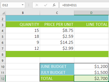
To create a formula:
In our example below, we'll use a simple formula and cell references to calculate a budget.
- Select the cell that will contain the formula. In our example, we'll select cell D12.

- Type the equals sign (=). Notice how it appears in both the cell and the formula bar.
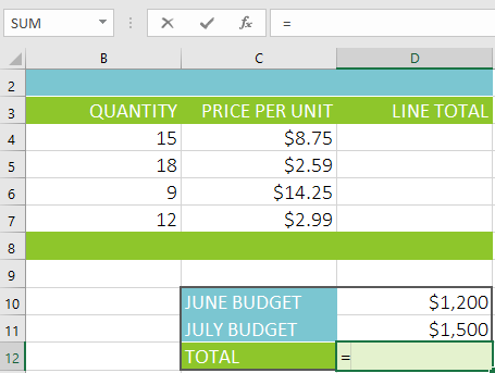
- Type the cell address of the cell you want to reference first in the formula: cell D10 in our example. A blue border will appear around the referenced cell.
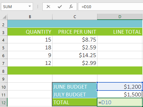
- Type the mathematical operator you want to use. In our example, we'll type the addition sign (+).
- Type the cell address of the cell you want to reference second in the formula: cell D11 in our example. A red border will appear around the referenced cell.
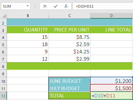
- Press Enter on your keyboard. The formula will be calculated, and the value will be displayed in the cell. If you select the cell again, notice that the cell displays the result, while the formula bar displays the formula.
If the result of a formula is too large to be displayed in a cell, it may appear as pound signs (#######) instead of a value. This means the column is not wide enough to display the cell content. Simply increase the column width to show the cell content.
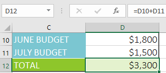
Modifying values with cell references
The true advantage of cell references is that they allow you to update data in your worksheet without having to rewrite formulas. In the example below, we've modified the value of cell D10 from $1,200 to $1,800. The formula in D12 will automatically recalculate and display the new value in cell D12.
Excel will not always tell you if your formula contains an error, so it's up to you to check all of your formulas. To learn how to do this, you can read the Double-Check Your Formulas lesson from our Excel Formulas tutorial.
To create a formula using the point-and-click method:
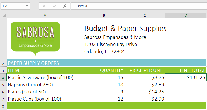
Instead of typing cell addresses manually, you can point and click the cells you want to include in your formula. This method can save a lot of time and effort when creating formulas. In our example below, we'll create a formula to calculate the cost of ordering several boxes of plastic silverware.
- Select the cell that will contain the formula. In our example, we'll select cell D4.

- Type the equals sign (=).
- Select the cell you want to reference first in the formula: cell B4 in our example. The cell address will appear in the formula.
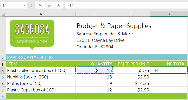
- Type the mathematical operator you want to use. In our example, we'll type the multiplication sign (*).
- Select the cell you want to reference second in the formula: cell C4 in our example. The cell address will appear in the formula.

- Press Enter on your keyboard. The formula will be calculated, and the value will be displayed in the cell.
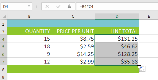
Copying formulas with the fill handle
Formulas can also be copied to adjacent cells with the fill handle, which can save a lot of time and effort if you need to perform the same calculation multiple times in a worksheet. The fill handle is the small square at the bottom-right corner of the selected cell(s).
- Select the cell containing the formula you want to copy. Click and drag the fill handle over the cells you want to fill.
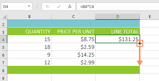
- After you release the mouse, the formula will be copied to the selected cells.
To edit a formula:
Sometimes you may want to modify an existing formula. In the example below, we've entered an incorrect cell address in our formula, so we'll need to correct it.
- Select the cell containing the formula you want to edit. In our example, we'll select cell D12.
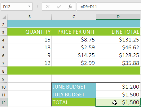
- Click the formula bar to edit the formula. You can also double-click the cell to view and edit the formula directly within the cell.

- A border will appear around any referenced cells. In our example, we'll change the first part of the formula to reference cell D10 instead of cell D9.
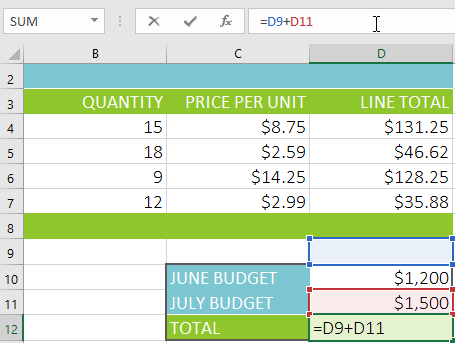
- When you're finished, press Enter on your keyboard or select the Enter command in the formula bar.
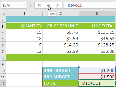
- The formula will be updated, and the new value will be displayed in the cell.
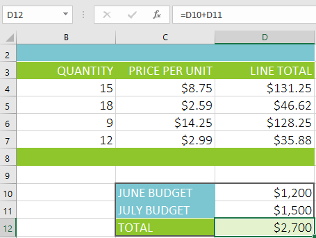
If you change your mind, you can press the Esc key on your keyboard or click the Cancel command in the formula bar to avoid accidentally making changes to your formula.
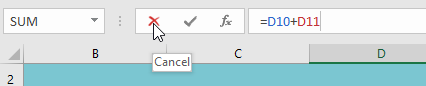
To show all of the formulas in a spreadsheet, you can hold the Ctrl key and press ` (grave accent). The grave accent key is usually located in the top-left corner of the keyboard. You can press Ctrl+` again to switch back to the normal view.
Challenge!
- Open our practice workbook.
- Click the Challenge tab in the bottom-left of the workbook.
- Create a formula in cell D4 that multiplies the quantity in B4 by the price per unit in cell C4.
- Use the fill handle to copy the formula in cell D4 to cells D5:D7.
- Change the price per unit for the fried plantains in cell C6 to $2.25. Notice that the line total automatically changes as well.
- Edit the formula for the total in cell D8 so it also adds cell D7.
- When you're finished, your workbook should look like this:
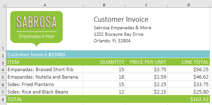
Lesson 14: Creating More Complex Formulas
Introduction
You may have experience working with formulas that contain only one operator, such as 7+9. More complex formulas can contain several mathematical operators, such as 5+2*8. When there's more than one operation in a formula, the order of operations tells Excel which operation to calculate first. To write formulas that will give you the correct answer, you'll need to understand the order of operations.
Optional: Download our practice workbook.
Watch the video below to learn more about complex formulas.
The order of operations
Excel calculates formulas based on the following order of operations:
- Operations enclosed in parentheses
- Exponential calculations (3^2, for example)
- Multiplication and division, whichever comes first
- Addition and subtraction, whichever comes first
A mnemonic that can help you remember the order is PEMDAS, or Please Excuse My Dear Aunt Sally.
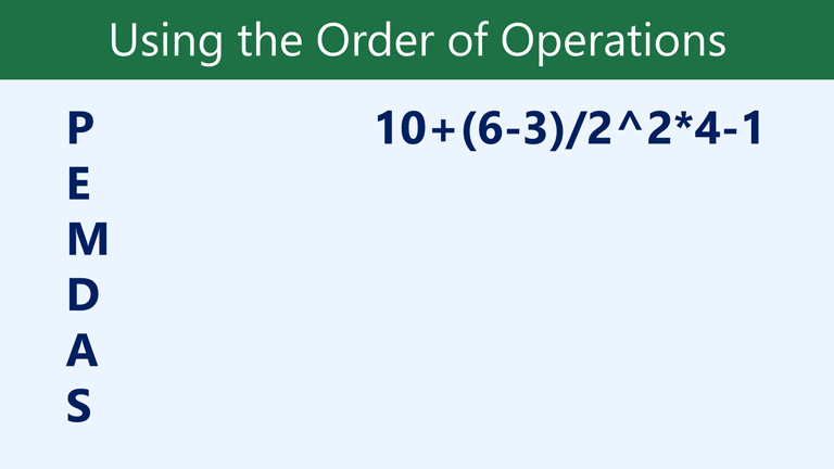
While this formula may look complicated, we can use the order of operations step by step to find the right answer.
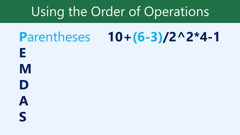
First, we'll start by calculating anything inside parentheses. In this case, there's only one thing we need to calculate: 6-3=3.
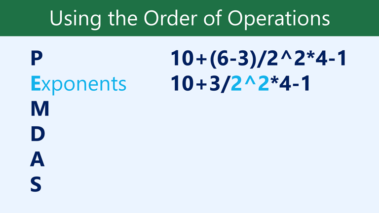
As you can see, the formula already looks simpler. Next, we'll look to see if there are any exponents. There is one: 2^2=4.
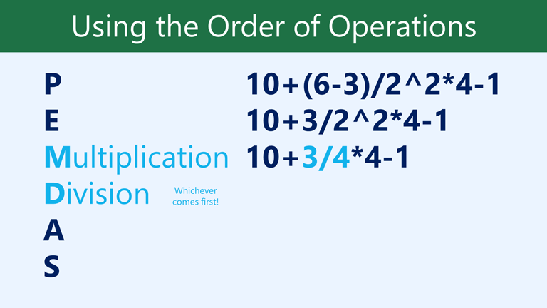
Next, we'll solve any multiplication and division, working from left to right. Because the division operation comes before the multiplication, it's calculated first: 3/4=0.75.
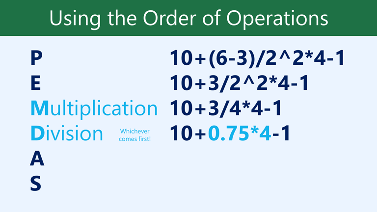
Now, we'll solve our remaining multiplication operation: 0.75*4=3.
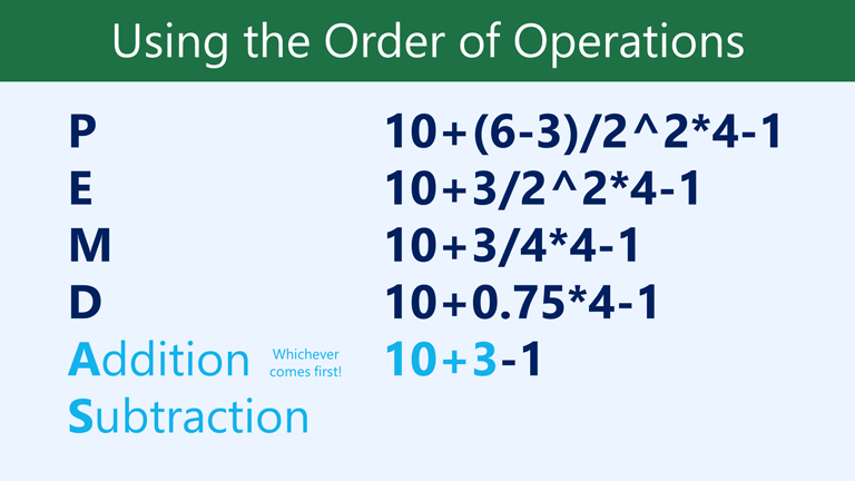
Next, we'll calculate any addition or subtraction, again working from left to right. Addition comes first: 10+3=13.
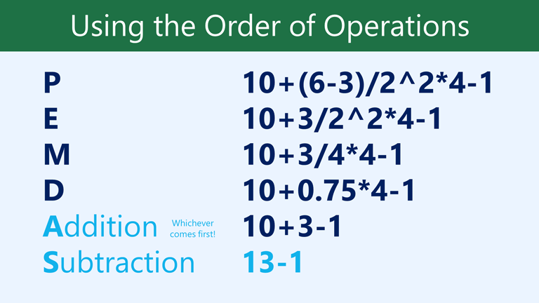
Finally, we have one remaining subtraction operation: 13-1=12.
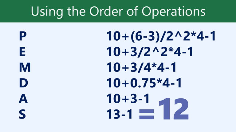
Now we have our answer: 12. And this is the exact same result you would get if you entered the formula into Excel.

Creating complex formulas
In the example below, we'll demonstrate how Excel uses the order of operations to solve a more complex formula. Here, we want to calculate the cost of sales tax for a catering invoice. To do this, we'll write our formula as =(D3+D4+D5)*0.075 in cell D6. This formula will add the prices of our items, then multiply that value by the 7.5% tax rate (which is written as 0.075) to calculate the answer.
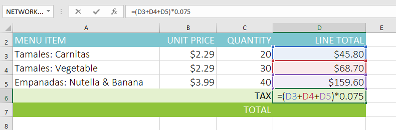
Excel follows the order of operations and first adds the values inside the parentheses: (45.80+68.70+159.60) = 274.10. It then multiplies that value by the tax rate: 274.10*0.075. The result will show that the sales tax is $20.56.
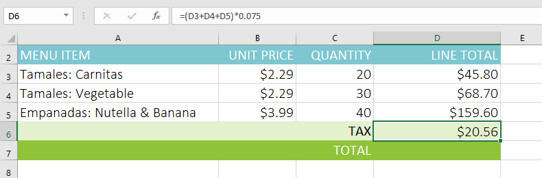
It's especially important to follow the order of operations when creating a formula. Otherwise, Excel won't calculate the results accurately. In our example, if the parentheses are not included, the multiplication is calculated first and the result is incorrect. Parentheses are often the best way to define which calculations will be performed first in Excel.
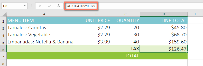
To create a complex formula using the order of operations:
In the example below, we'll use cell references along with numerical values to create a complex formula that will calculate the subtotal for a catering invoice. The formula will calculate the cost of each menu item first, then add these values.
- Select the cell that will contain the formula. In our example, we'll select cell C5.
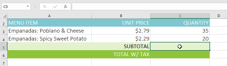
- Enter your formula. In our example, we'll type =B3*C3+B4*C4. This formula will follow the order of operations, first performing the multiplication: 2.79*35 = 97.65 and 2.29*20 = 45.80. It then will add these values to calculate the total: 97.65+45.80.

- Double-check your formula for accuracy, then press Enter on your keyboard. The formula will calculate and display the result. In our example, the result shows that the subtotal for the order is $143.45.
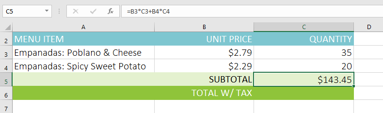
You can add parentheses to any equation to make it easier to read. While it won't change the result of the formula in this example, we could enclose the multiplication operations within parentheses to clarify that they will be calculated before the addition.
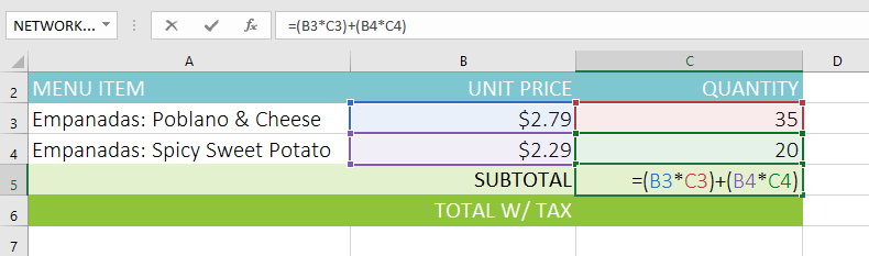
Excel will not always tell you if your formula contains an error, so it's up to you to check all of your formulas. To learn how to do this, you can read the Double-Check Your Formulas lesson from our Excel Formulas tutorial.
Challenge!
For this challenge, you are going to work with another invoice like the one in our example. In the invoice, you will find the amount of tax for the order, the order's total, and the order's total if you were given a 10% discount.
- Open our practice workbook.
- Click the Challenge worksheet tab in the bottom-left of the workbook.
- In cell D7, create a formula that calculates the tax for the invoice. Use a sales tax rate of 7.5%.
- In cell D8, create a formula that finds the total for the order. In other words, this formula should add cells D3:D7.
- In cell D9 create a formula that calculates the total after a 10% discount. If you need help understanding how to take a percentage off of a total, check out our lesson on Discounts, Markdowns, and Sales.
- When you're finished, your spreadsheet should look like this:
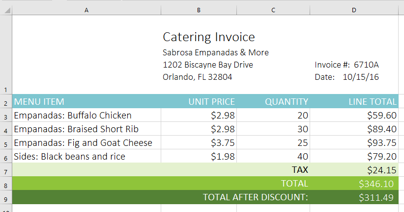
Lesson 15: Relative and Absolute Cell References
Introduction
There are two types of cell references: relative and absolute. Relative and absolute references behave differently when copied and filled to other cells. Relative references change when a formula is copied to another cell. Absolute references, on the other hand, remain constant no matter where they are copied.
Optional: Download our practice workbook.
Watch the video below to learn more about cell references.
Relative references
By default, all cell references are relative references. When copied across multiple cells, they change based on the relative position of rows and columns. For example, if you copy the formula =A1+B1 from row 1 to row 2, the formula will become =A2+B2. Relative references are especially convenient whenever you need to repeat the same calculation across multiple rows or columns.
To create and copy a formula using relative references:
In the following example, we want to create a formula that will multiply each item's price by the quantity. Instead of creating a new formula for each row, we can create a single formula in cell D4 and then copy it to the other rows. We'll use relative references so the formula calculates the total for each item correctly.
- Select the cell that will contain the formula. In our example, we'll select cell D4.
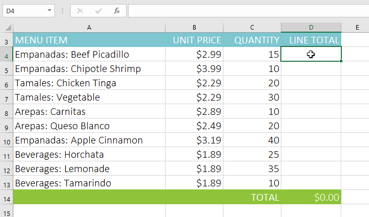
- Enter the formula to calculate the desired value. In our example, we'll type =B4*C4.
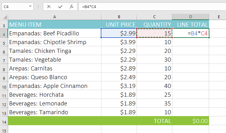
- Press Enter on your keyboard. The formula will be calculated, and the result will be displayed in the cell.
- Locate the fill handle in the bottom-right corner of the desired cell. In our example, we'll locate the fill handle for cell D4.
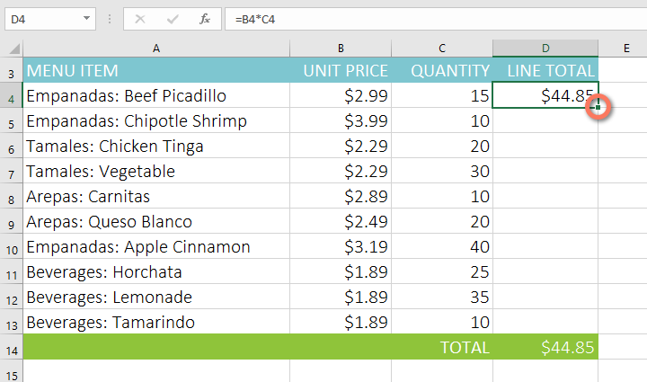
- Click and drag the fill handle over the cells you want to fill. In our example, we'll select cells D5:D13.
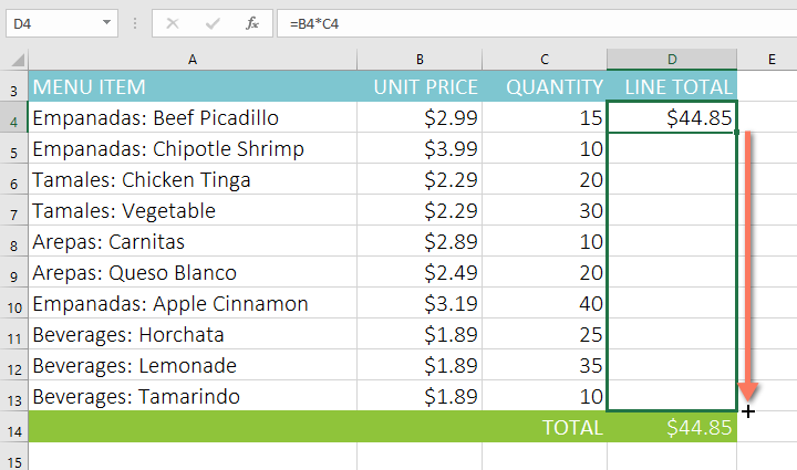
- Release the mouse. The formula will be copied to the selected cells with relative references, displaying the result in each cell.
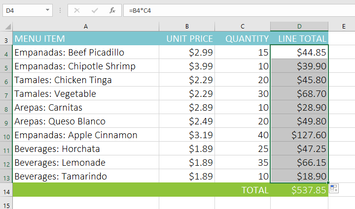
You can double-click the filled cells to check their formulas for accuracy. The relative cell references should be different for each cell, depending on their rows.
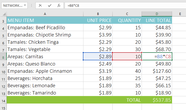
Absolute references
There may be times when you do not want a cell reference to change when filling cells. Unlike relative references, absolute references do not change when copied or filled. You can use an absolute reference to keep a row and/or column constant.
An absolute reference is designated in a formula by the addition of a dollar sign ($) before the column and row. If it precedes the column or row (but not both), it's known as a mixed reference.
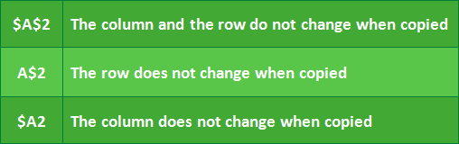
You will use the relative (A2) and absolute ($A$2) formats in most formulas. Mixed references are used less frequently.
When writing a formula in Microsoft Excel, you can press the F4 key on your keyboard to switch between relative, absolute, and mixed cell references, as shown in the video below. This is an easy way to quickly insert an absolute reference.
To create and copy a formula using absolute references:
In the example below, we're going to use cell E2 (which contains the tax rate at 7.5%) to calculate the sales tax for each item in column D. To make sure the reference to the tax rate stays constant—even when the formula is copied and filled to other cells—we'll need to make cell $E$2 an absolute reference.
- Select the cell that will contain the formula. In our example, we'll select cell D4.
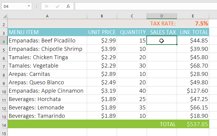
- Enter the formula to calculate the desired value. In our example, we'll type =(B4*C4)*$E$2, making $E$2 an absolute reference.
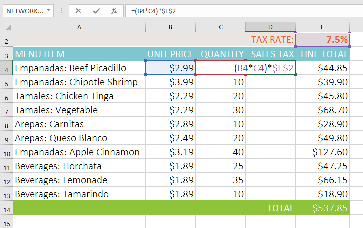
- Press Enter on your keyboard. The formula will calculate, and the result will display in the cell.
- Locate the fill handle in the bottom-right corner of the desired cell. In our example, we'll locate the fill handle for cell D4.
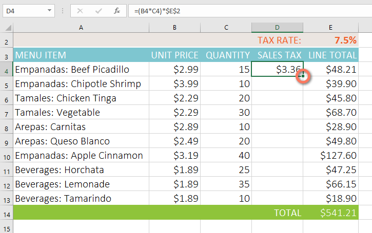
- Click and drag the fill handle over the cells you want to fill (cells D5:D13 in our example).
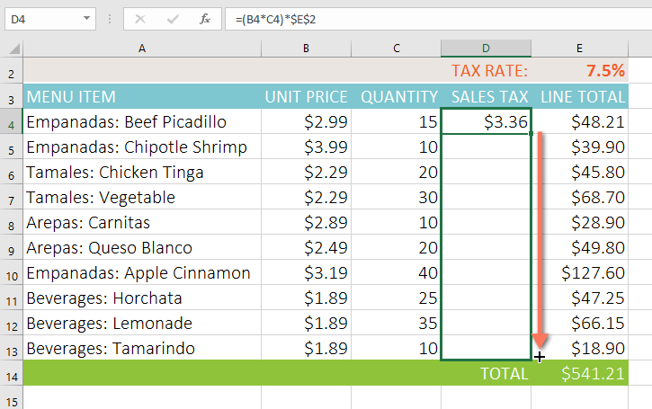
- Release the mouse. The formula will be copied to the selected cells with an absolute reference, and the values will be calculated in each cell.
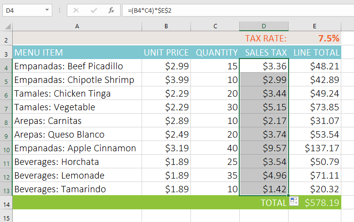
You can double-click the filled cells to check their formulas for accuracy. The absolute reference should be the same for each cell, while the other references are relative to the cell's row.
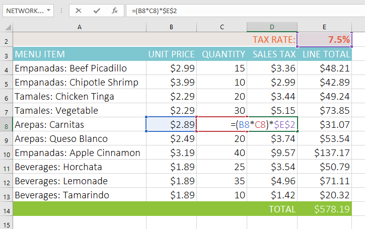
Be sure to include the dollar sign ($) whenever you're making an absolute reference across multiple cells. The dollar signs were omitted in the example below. This caused Excel to interpret it as a relative reference, producing an incorrect result when copied to other cells.
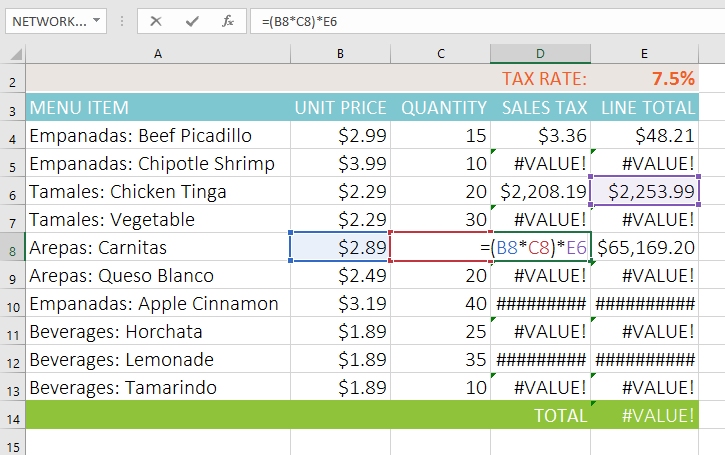
Using cell references with multiple worksheets
Excel allows you to refer to any cell on any worksheet, which can be especially helpful if you want to reference a specific value from one worksheet to another. To do this, you'll simply need to begin the cell reference with the worksheet name followed by an exclamation point (!). For example, if you wanted to reference cell A1 on Sheet1, its cell reference would be Sheet1!A1.
Note that if a worksheet name contains a space, you'll need to include single quotation marks (' ') around the name. For example, if you wanted to reference cell A1 on a worksheet named July Budget, its cell reference would be 'July Budget'!A1.
To reference cells across worksheets:
In our example below, we'll refer to a cell with a calculated value between two worksheets. This will allow us to use the exact same value on two different worksheets without rewriting the formula or copying data.
- Locate the cell you want to reference, and note its worksheet. In our example, we want to reference cell E14 on the Menu Order worksheet.
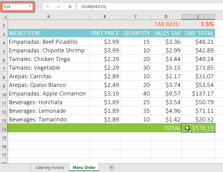
- Navigate to the desired worksheet. In our example, we'll select the Catering Invoice worksheet.
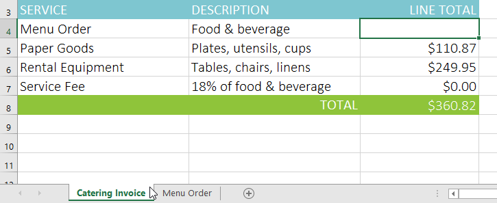
- Locate and select the cell where you want the value to appear. In our example, we'll select cell C4.

- Type the equals sign (=), the sheet name followed by an exclamation point (!), and the cell address. In our example, we'll type ='Menu Order'!E14.
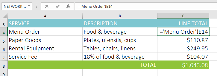
- Press Enter on your keyboard. The value of the referenced cell will appear. Now, if the value of cell E14 changes on the Menu Order worksheet, it will be updated automatically on the Catering Invoice worksheet.
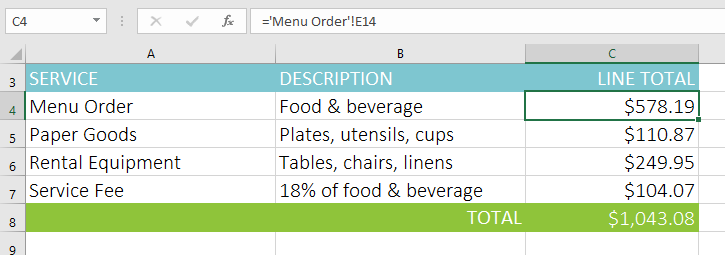
If you rename your worksheet at a later point, the cell reference will be updated automatically to reflect the new worksheet name.
If you enter a worksheet name incorrectly, the #REF! error will appear in the cell. In our example below, we've mistyped the name of the worksheet. To edit, ignore, or investigate the error, click the Error button beside the cell and choose an option from the menu.
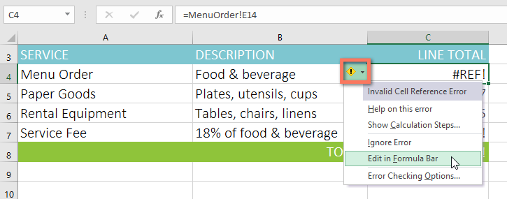
Challenge!
- Open our practice workbook.
- Click the Paper Goods tab in the bottom-left of the workbook.
- In cell D4, enter a formula that multiplies the unit price in B4, the quantity in C4, and the tax rate in E2. Make sure to use an absolute cell reference for the tax rate because it will be the same in every cell.
- Use the fill handle to copy the formula you just created to cells D5:D12.
- Change the tax rate in cell E2 to 6.5%. Notice that all of your cells have updated. When you're finished, your workbook should look like this:
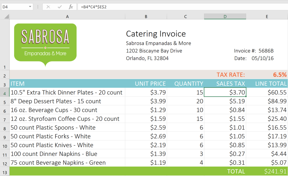
- Click the Catering Invoice tab.
- Delete the value in cell C5 and replace it with a reference to the total cost of the paper goods. Hint: The cost of the paper goods is in cell E13 on the Paper Goods worksheet.
- Use the same steps from above to calculate the sales tax for each item on the Menu Order worksheet. The total cost in cell E14 should update. Then, in cell C4 of the Catering Invoice worksheet, create a cell reference to the total you just calculated. Note: If you used our practice workbook to follow along during the lesson, you may have already completed this step.
- When you're finished, the Catering Invoice worksheet should look something like this:
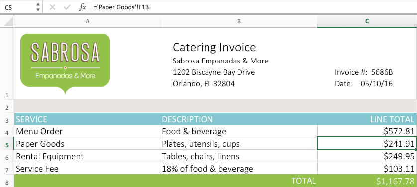
Lesson 16: Functions
Introduction
A function is a predefined formula that performs calculations using specific values in a particular order. Excel includes many common functions that can be used to quickly find the sum, average, count, maximum value, and minimum value for a range of cells. In order to use functions correctly, you'll need to understand the different parts of a function and how to create arguments to calculate values and cell references.
Optional: Download our practice workbook.
Watch the video below to learn more about working with functions.
The parts of a function
In order to work correctly, a function must be written a specific way, which is called the syntax. The basic syntax for a function is the equals sign (=), the function name (SUM, for example), and one or more arguments. Arguments contain the information you want to calculate. The function in the example below would add the values of the cell range A1:A20.

Working with arguments
Arguments can refer to both individual cells and cell ranges and must be enclosed within parentheses. You can include one argument or multiple arguments, depending on the syntax required for the function.
For example, the function =AVERAGE(B1:B9) would calculate the average of the values in the cell range B1:B9. This function contains only one argument.
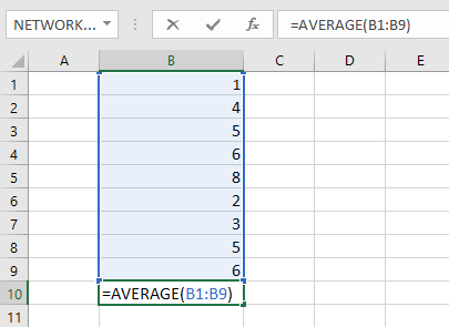
Multiple arguments must be separated by a comma. For example, the function =SUM(A1:A3, C1:C2, E1) will add the values of all of the cells in the three arguments.
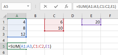
Creating a function
There are a variety of functions available in Excel. Here are some of the most common functions you'll use:
- SUM: This function adds all of the values of the cells in the argument.
- AVERAGE: This function determines the average of the values included in the argument. It calculates the sum of the cells and then divides that value by the number of cells in the argument.
- COUNT: This function counts the number of cells with numerical data in the argument. This function is useful for quickly counting items in a cell range.
- MAX: This function determines the highest cell value included in the argument.
- MIN: This function determines the lowest cell value included in the argument.
To create a function using the AutoSum command:
The AutoSum command allows you to automatically insert the most common functions into your formula, including SUM, AVERAGE, COUNT, MIN, and MAX. In the example below, we'll use the SUM function to calculate the total cost for a list of recently ordered items.
- Select the cell that will contain the function. In our example, we'll select cell D13.
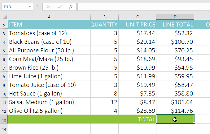
- In the Editing group on the Home tab, click the arrow next to the AutoSum command. Next, choose the desired function from the drop-down menu. In our example, we'll select Sum.
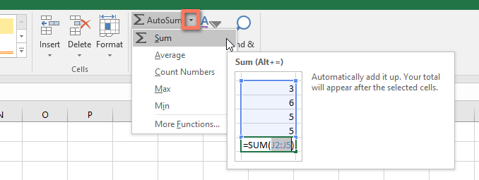
- Excel will place the function in the cell and automatically select a cell range for the argument. In our example, cells D3:D12 were selected automatically; their values will be added to calculate the total cost. If Excel selects the wrong cell range, you can manually enter the desired cells into the argument.
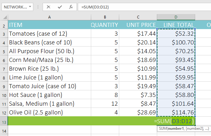
- Press Enter on your keyboard. The function will be calculated, and the result will appear in the cell. In our example, the sum of D3:D12 is $765.29.
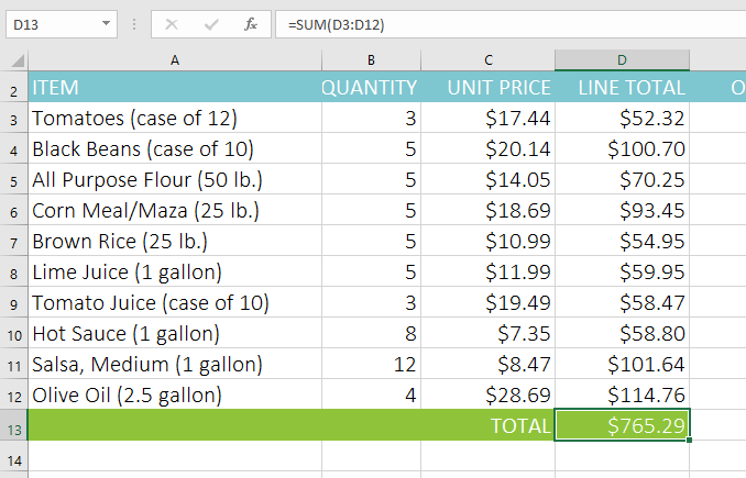
The AutoSum command can also be accessed from the Formulas tab on the Ribbon.
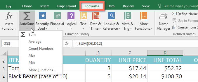
You can also use the Alt+= keyboard shortcut instead of the AutoSum command. To use this shortcut, hold down the Alt key and then press the equals sign.
Watch the video below to see this shortcut in action.
To enter a function manually:
If you already know the function name, you can easily type it yourself. In the example below (a tally of cookie sales), we'll use the AVERAGE function to calculate the average number of units sold by each troop.
- Select the cell that will contain the function. In our example, we'll select cell C10.
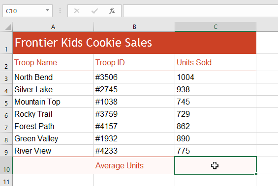
- Type the equals sign (=), and enter the desired function name. You can also select the desired function from the list of suggested functions that appears below the cell as you type. In our example, we'll type =AVERAGE.
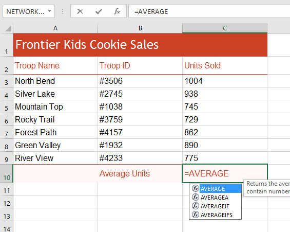
- Enter the cell range for the argument inside parentheses. In our example, we'll type (C3:C9). This formula will add the values of cells C3:C9, then divide that value by the total number of values in the range.
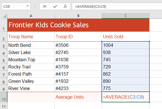
- Press Enter on your keyboard. The function will be calculated, and the result will appear in the cell. In our example, the average number of units sold by each troop is 849.
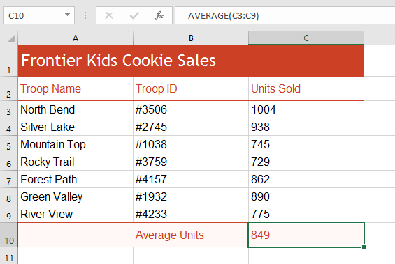
Excel will not always tell you if your formula contains an error, so it's up to you to check all of your formulas. To learn how to do this, read the Double-Check Your Formulas lesson from our Excel Formulas tutorial.
The Function Library
While there are hundreds of functions in Excel, the ones you'll use the most will depend on the type of data your workbooks contain. There's no need to learn every single function, but exploring some of the different types of functions will help you as you create new projects. You can even use the Function Library on the Formulas tab to browse functions by category, such as Financial, Logical, Text, and Date & Time.
To access the Function Library, select the Formulas tab on the Ribbon. Look for the Function Library group.
Click the buttons in the interactive below to learn more about the different types of functions in Excel.
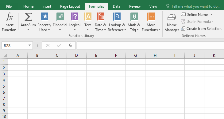
Lookup & Reference
The Lookup & Reference category contains functions that will return results for finding and referencing information. For example, you can add a hyperlink to a cell (HYPERLINK) or return the value of a particular row and column intersection (INDEX).
To insert a function from the Function Library:
In the example below, we'll use the COUNTA function to count the total number of items in the Items column. Unlike COUNT, COUNTA can be used to tally cells that contain data of any kind, not just numerical data.
- Select the cell that will contain the function. In our example, we'll select cell B17.
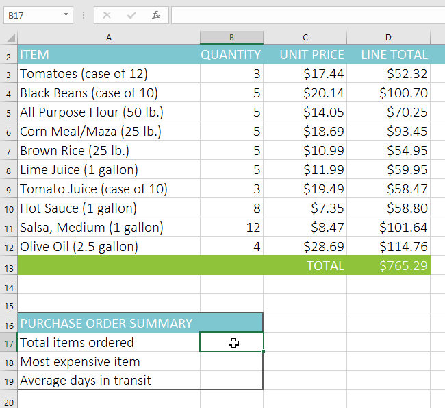
- Click the Formulas tab on the Ribbon to access the Function Library.
- From the Function Library group, select the desired function category. In our example, we'll choose More Functions, then hover the mouse over Statistical.

- Select the desired function from the drop-down menu. In our example, we'll select the COUNTA function, which will count the number of cells in the Items column that are not empty.
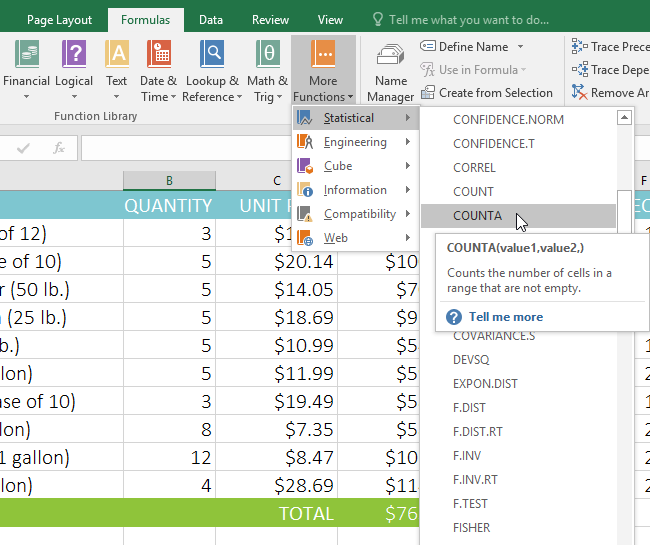
- The Function Arguments dialog box will appear. Select the Value1 field, then enter or select the desired cells. In our example, we'll enter the cell range A3:A12. You may continue to add arguments in the Value2 field, but in this case we only want to count the number of cells in the cell range A3:A12.
- When you're satisfied, click OK.
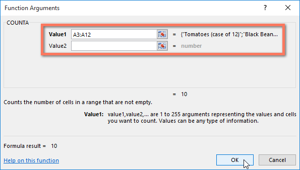
- The function will be calculated, and the result will appear in the cell. In our example, the result shows that a total of 10 items were ordered.
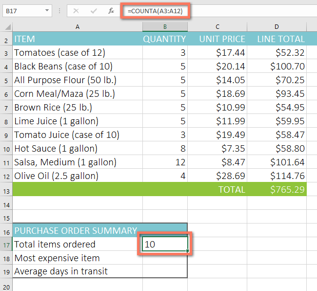
The Insert Function command
While the Function Library is a great place to browse for functions, sometimes you may prefer to search for one instead. You can do so using the Insert Function command. It may take some trial and error depending on the type of function you're looking for; however, with practice, the Insert Function command can be a powerful way to find a function quickly.
To use the Insert Function command:
In the example below, we want to find a function that will calculate the number of business days it took to receive items after they were ordered. We'll use the dates in columns E and F to calculate the delivery time in column G.
- Select the cell that will contain the function. In our example, we'll select cell G3.
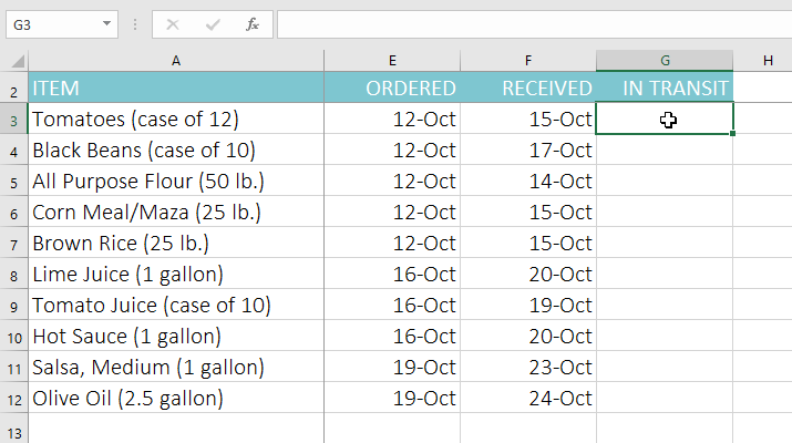
- Click the Formulas tab on the Ribbon, then click the Insert Function command.
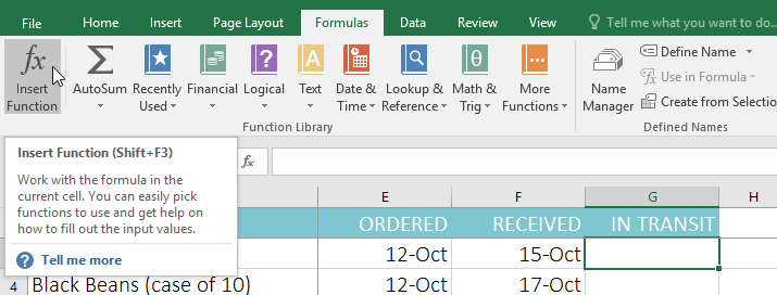
- The Insert Function dialog box will appear.
- Type a few keywords describing the calculation you want the function to perform, then click Go. In our example, we'll type count days, but you can also search by selecting a category from the drop-down list.
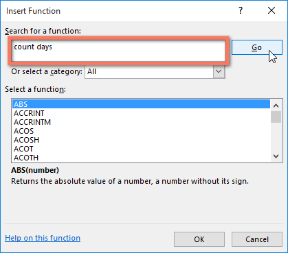
- Review the results to find the desired function, then click OK. In our example, we'll choose NETWORKDAYS, which will count the number of business days between the ordered date and received date.
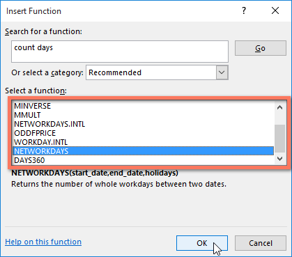
- The Function Arguments dialog box will appear. From here, you'll be able to enter or select the cells that will make up the arguments in the function. In our example, we'll enter E3 in the Start_date field and F3 in the End_date field.
- When you're satisfied, click OK.
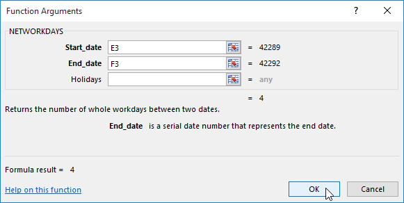
- The function will be calculated, and the result will appear in the cell. In our example, the result shows that it took four business days to receive the order.
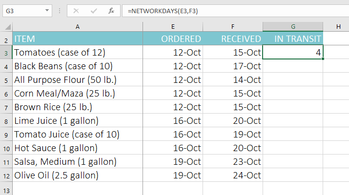
Like formulas, functions can be copied to adjacent cells. Simply select the cell that contains the function, then click and drag the fill handle over the cells you want to fill. The function will be copied, and values for those cells will be calculated relative to their rows or columns.
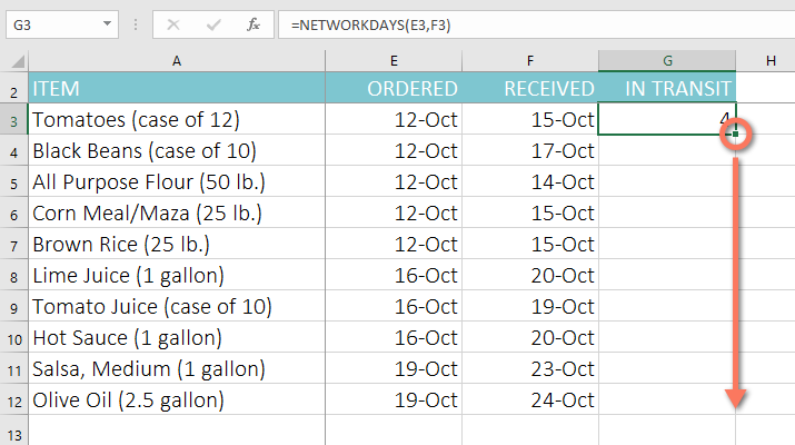
To learn more:
If you're comfortable with basic functions, you may want to try a more advanced one like VLOOKUP. Check out our article on How to Use Excel's VLOOKUP Function for more information.
To learn even more about working with functions, visit our Excel Formulas tutorial.
Challenge!
- Open our practice workbook.
- Click the Challenge tab in the bottom-left of the workbook.
- In cell F3, insert a function to calculate the average of the four scores in cells B3:E3.
- Use the fill handle to copy your function in cell F3 to cells F4:F17.
- In cell B18, use AutoSum to insert a function that calculates the lowest score in cells B3:B17.
- In cell B19, use the Function Library to insert a function that calculates the median of the scores in cells B3:B17. Hint: You can find the median function by going to More Functions > Statistical.
- In cell B20, create a function to calculate the highest score in cells B3:B17.
- Select cells B18:B20, then use the fill handle to copy all three functions you just created to cells C18:F20.
- When you're finished, your workbook should look like this:
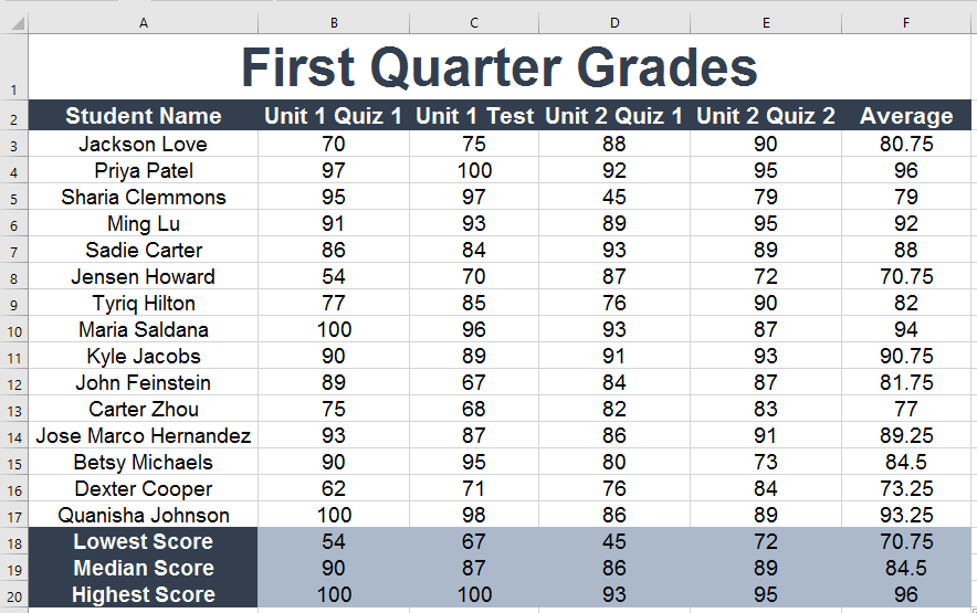
Lesson 17: Basic Tips for Working with Data
Introduction
Excel workbooks are designed to store a lot of information. Whether you're working with 20 cells or 20,000, Excel has several features to help you organize your data and find what you need. You can see some of the most useful features below. And be sure to check out the other lessons in this tutorial to get step-by-step instructions for each of these features.
Freezing rows and columns
You may want to see certain rows or columns all the time in your worksheet, especially header cells. By freezing rows or columns in place, you'll be able to scroll through your content while continuing to view the frozen cells. In this example, we've frozen the top two rows, which allows us to view the dates no matter where we scroll in the spreadsheet.
Sorting data
You can quickly reorganize a worksheet by sorting your data. Content can be sorted alphabetically, numerically, and in many other ways. For example, you could organize a list of contact information by last name.
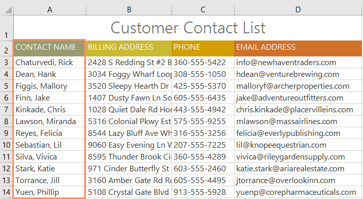
Filtering data
Filters can be used to narrow down the data in your worksheet, allowing you to view only the information you need. In this example, we're filtering the worksheet to show only rows that contain the words Laptop or Projector in column B.

Summarizing data
The Subtotal feature allows you to quickly summarize your data. In our example, we've created a subtotal for each T-shirt size, which makes it easy to see how many we'll need in each size.

Formatting data as a table
Just like regular formatting, tables can improve the look and feel of your workbook, but they'll also help you organize your content and make your data easier to use. For example, tables have built-in sorting and filtering options. Excel also includes several predefined table styles, allowing you to create tables quickly.

Visualizing data with charts
It can be difficult to interpret Excel workbooks that contain a lot of data. Charts allow you to illustrate your workbook data graphically, which makes it easy to visualize comparisons and trends.
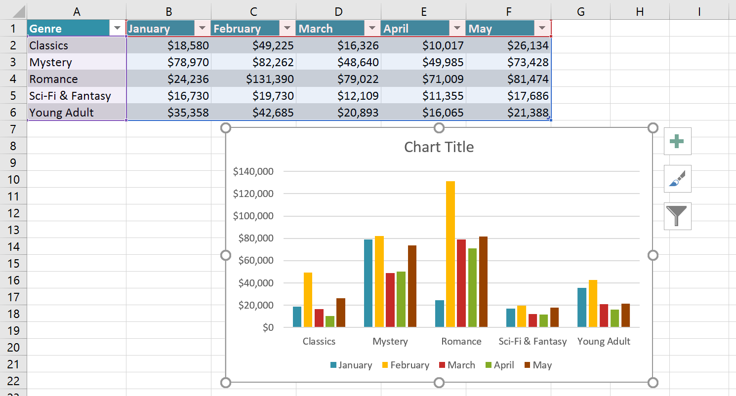
Adding conditional formatting
Let's say you have a worksheet with thousands of rows of data. It would be extremely difficult to see patterns and trends just from examining the raw information. Conditional formatting allows you to automatically apply cell formatting—such as colors, icons, and data bars—to one or more cells based on the cell value.
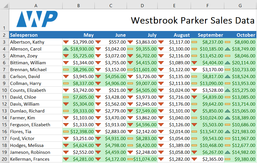
Using Find and Replace
When working with a lot of data, it can be difficult and time consuming to locate specific information. You can easily search your workbook using the Find feature, which also allows you to modify content using the Replace feature.

Lesson 18: Freezing Panes and View Options
Introduction
Whenever you're working with a lot of data, it can be difficult to compare information in your workbook. Fortunately, Excel includes several tools that make it easier to view content from different parts of your workbook at the same time, including the ability to freeze panes and split your worksheet.
Optional: Download our practice workbook.
Watch the video below to learn more about freezing panes in Excel.
To freeze rows:
You may want to see certain rows or columns all the time in your worksheet, especially header cells. By freezing rows or columns in place, you'll be able to scroll through your content while continuing to view the frozen cells.
- Select the row below the row(s) you want to freeze. In our example, we want to freeze rows 1 and 2, so we'll select row 3.
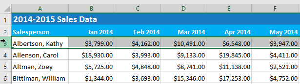
- On the View tab, select the Freeze Panes command, then choose Freeze Panes from the drop-down menu.
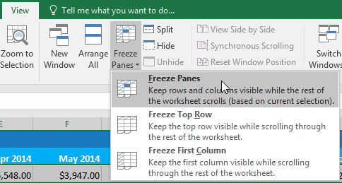
- The rows will be frozen in place, as indicated by the gray line. You can scroll down the worksheet while continuing to view the frozen rows at the top. In our example, we've scrolled down to row 18.

To freeze columns:
- Select the column to the right of the column(s) you want to freeze. In our example, we want to freeze column A, so we'll select column B.
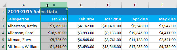
- On the View tab, select the Freeze Panes command, then choose Freeze Panes from the drop-down menu.
- The column will be frozen in place, as indicated by the gray line. You can scroll across the worksheet while continuing to view the frozen column on the left. In our example, we've scrolled across to column E.
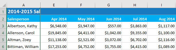
If you only need to freeze the top row (row 1) or first column (column A) in the worksheet, you can simply select Freeze Top Row or Freeze First Column from the drop-down menu.
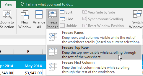
To unfreeze panes:
If you want to select a different view option, you may first need to reset the spreadsheet by unfreezing panes. To unfreeze rows or columns, click the Freeze Panes command, then select Unfreeze Panes from the drop-down menu.
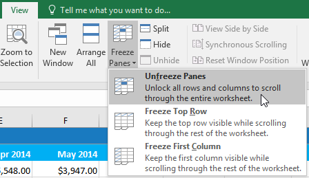
Other view options
If your workbook contains a lot of content, it can sometimes be difficult to compare different sections. Excel includes additional options to make your workbooks easier to view and compare. For example, you can choose to open a new window for your workbook or split a worksheet into separate panes.
To open a new window for the current workbook:
Excel allows you to open multiple windows for a single workbook at the same time. In our example, we'll use this feature to compare two different worksheets from the same workbook.
- Click the View tab on the Ribbon, then select the New Window command.
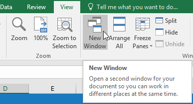
- A new window for the workbook will appear.
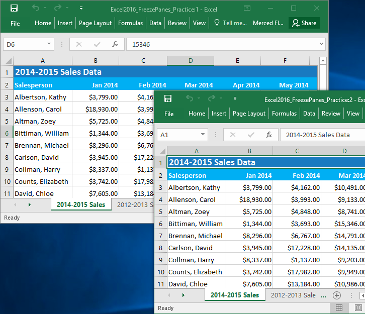
- You can now compare different worksheets from the same workbook across windows. In our example, we'll select the 2013 Sales Detailed View worksheet to compare 2012 and 2013 sales.
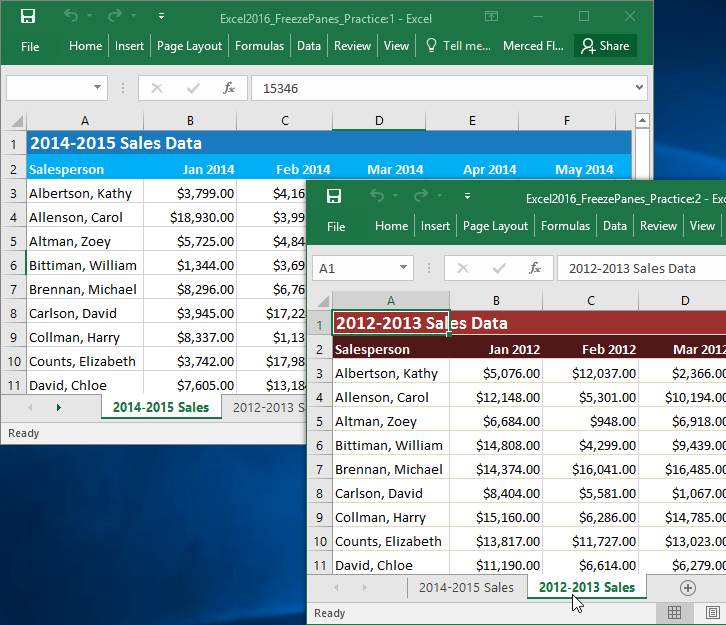
If you have several windows open at the same time, you can use the Arrange All command to rearrange them quickly.
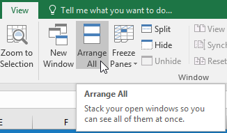
To split a worksheet:
Sometimes you may want to compare different sections of the same workbook without creating a new window. The Split command allows you to divide the worksheet into multiple panes that scroll separately.
- Select the cell where you want to split the worksheet. In our example, we'll select cell D6.
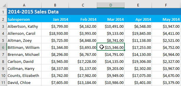
- Click the View tab on the Ribbon, then select the Split command.
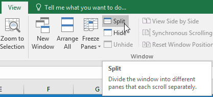
- The workbook will be split into different panes. You can scroll through each pane separately using the scroll bars, allowing you to compare different sections of the workbook.
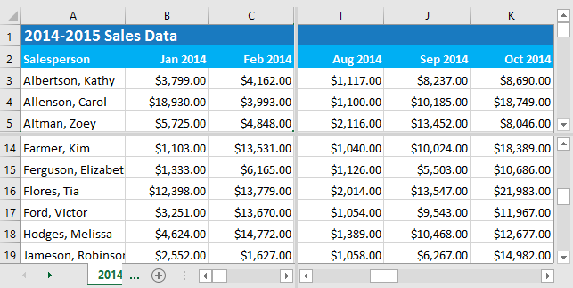
- After creating a split, you can click and drag the vertical and horizontal dividers to change the size of each section.
To remove the split, click the Split command again.
Challenge!
Within our example file, there is A LOT of sales data. For this challenge, we want to be able to compare data for different years side by side. To do this:
- Open our practice workbook.
- Open a new window for your workbook.
- Freeze First Column and use the horizontal scroll bar to look at sales from 2015.
- Unfreeze the first column.
- Select cell G17 and click Split to split the worksheet into multiple panes. Hint: This should split the worksheet between rows 16 and 17 and columns F and G.
- Use the horizontal scroll bar in the bottom right of the window to move the worksheet so that Column N, which contains data for January 2015, is next to Column F.
- Open a new window for your workbook, and select the 2012-2013 Sales tab.
- Move your windows so they are side by side. Now you're able to compare data for similar months from several different years. Your screen should look something like this:
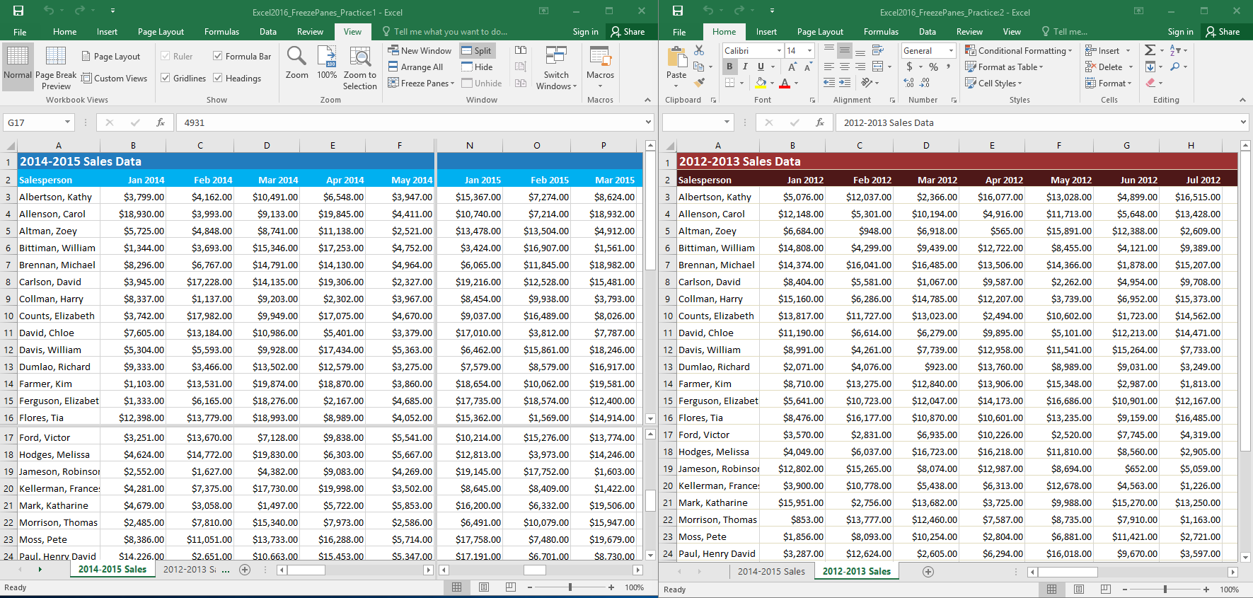
Lesson 19: Sorting Data
Introduction
As you add more content to a worksheet, organizing this information becomes especially important. You can quickly reorganize a worksheet by sorting your data. For example, you could organize a list of contact information by last name. Content can be sorted alphabetically, numerically, and in many other ways.
Optional: Download our practice workbook.
Watch the video below to learn more about sorting data in Excel.
Types of sorting
When sorting data, it's important to first decide if you want the sort to apply to the entire worksheet or just a cell range.
- Sort sheet organizes all of the data in your worksheet by one column. Related information across each row is kept together when the sort is applied. In the example below, the Contact Name column (column A) has been sorted to display the names in alphabetical order.

- Sort range sorts the data in a range of cells, which can be helpful when working with a sheet that contains several tables. Sorting a range will not affect other content on the worksheet.
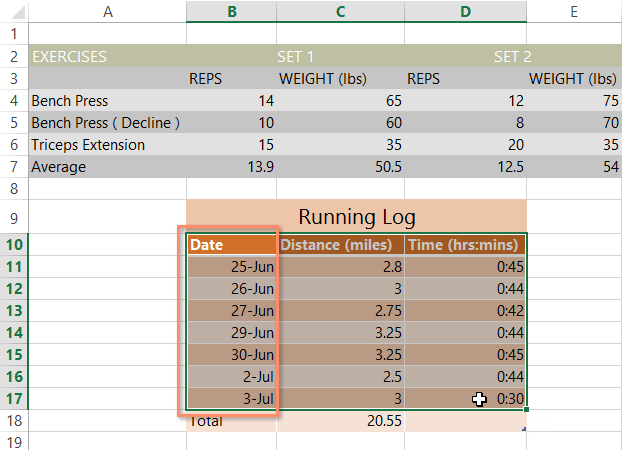
To sort a sheet:
In our example, we'll sort a T-shirt order form alphabetically by Last Name (column C).
- Select a cell in the column you want to sort by. In our example, we'll select cell C2.
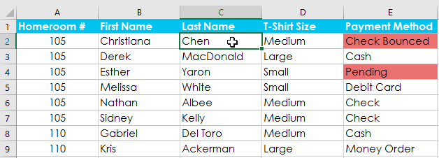
- Select the Data tab on the Ribbon, then click the A-Z command to sort A to Z, or the Z-A command to sort Z to A. In our example, we'll sort A to Z.
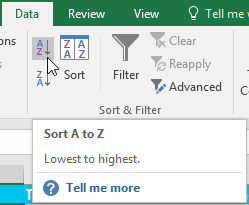
- The worksheet will be sorted by the selected column. In our example, the worksheet is now sorted by last name.
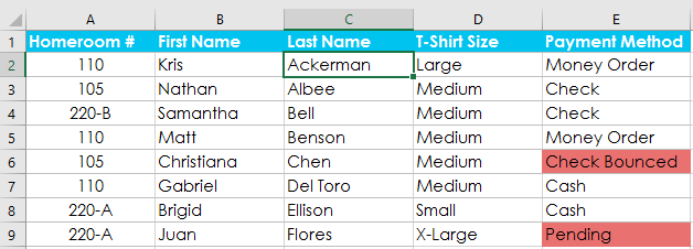
To sort a range:
In our example, we'll select a separate table in our T-shirt order form to sort the number of shirts that were ordered in each grade.
- Select the cell range you want to sort. In our example, we'll select cell range G2:H6.
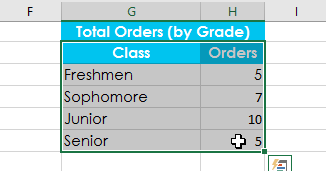
- Select the Data tab on the Ribbon, then click the Sort command.
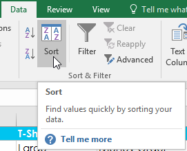
- The Sort dialog box will appear. Choose the column you want to sort by. In our example, we want to sort the data by the number of T-shirt orders, so we'll select Orders.

- Decide the sorting order (either ascending or descending). In our example, we'll use Largest to Smallest.
- Once you're satisfied with your selection, click OK.
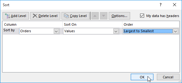
- The cell range will be sorted by the selected column. In our example, the Orders column will be sorted from highest to lowest. Notice that the other content in the worksheet was not affected by the sort.
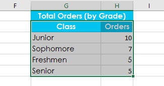
If your data isn't sorting properly, double-check your cell values to make sure they are entered into the worksheet correctly. Even a small typo could cause problems when sorting a large worksheet. In the example below, we forgot to include a hyphen in cell A18, causing our sort to be slightly inaccurate.
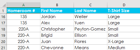
Custom sorting
Sometimes you may find that the default sorting options can't sort data in the order you need. Fortunately, Excel allows you to create a custom list to define your own sorting order.
To create a custom sort:
In our example below, we want to sort the worksheet by T-Shirt Size (column D). A regular sort would organize the sizes alphabetically, which would be incorrect. Instead, we'll create a custom list to sort from smallest to largest.
- Select a cell in the column you want to sort by. In our example, we'll select cell D2.
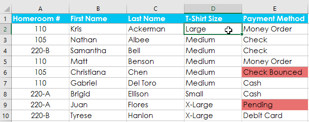
- Select the Data tab, then click the Sort command.
- The Sort dialog box will appear. Select the column you want to sort by, then choose Custom List... from the Order field. In our example, we will choose to sort by T-Shirt Size.
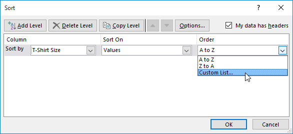
- The Custom Lists dialog box will appear. Select NEW LIST from the Custom Lists: box.
- Type the items in the desired custom order in the List entries: box. In our example, we want to sort our data by T-shirt size from smallest to largest, so we'll type Small, Medium, Large, and X-Large, pressing Enter on the keyboard after each item.
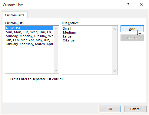
- Click Add to save the new sort order. The new list will be added to the Custom lists: box. Make sure the new list is selected, then click OK.
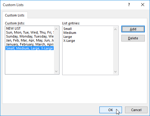
- The Custom Lists dialog box will close. Click OK in the Sort dialog box to perform the custom sort.

- The worksheet will be sorted by the custom order. In our example, the worksheet is now organized by T-shirt size from smallest to largest.
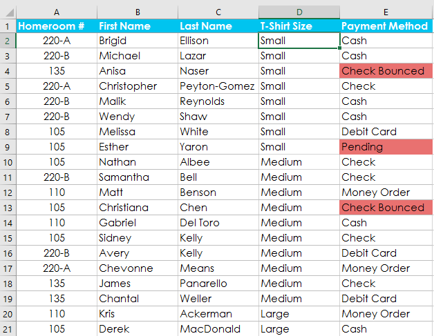
Sorting levels
If you need more control over how your data is sorted, you can add multiple levels to any sort. This allows you to sort your data by more than one column.
To add a level:
In our example below, we'll sort the worksheet by T-Shirt Size (Column D), and then by Homeroom Number (column A).
- Select a cell in the column you want to sort by. In our example, we'll select cell A2.
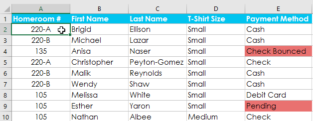
- Click the Data tab, then select the Sort command.
- The Sort dialog box will appear. Select the first column you want to sort by. In this example, we will sort by T-Shirt Size (column D) with the custom list we previously created for the Order field.
- Click Add Level to add another column to sort by.
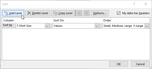
- Select the next column you want to sort by, then click OK. In our example, we'll sort by Homeroom # (column A).
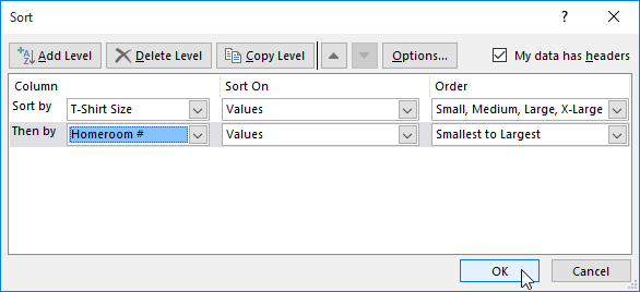
- The worksheet will be sorted according to the selected order. In our example, the orders are sorted by T-shirt size. Within each group of T-shirt sizes, students are sorted by homeroom number.
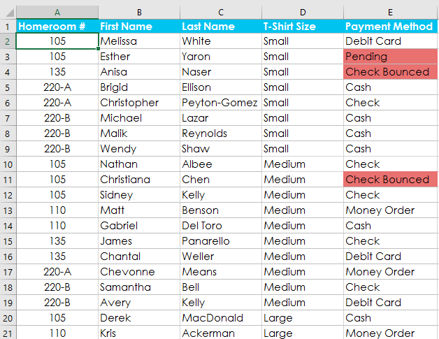
If you need to change the order of a multilevel sort, it's easy to control which column is sorted first. Simply select the desired column, then click the Move Up or Move Down arrow to adjust its priority.
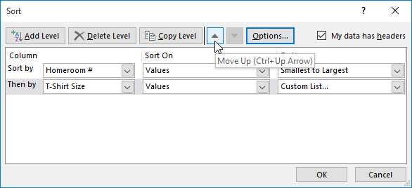
Challenge!
- Open our practice workbook.
- Click the Challenge tab in the bottom-left of the workbook.
- For the main table, create a custom sort that sorts by Grade from Smallest to Largest and then by Camper Name from A to Z.
- Create a sort for the Additional Information section. Sort by Counselor (Column H) from A to Z.
- When you're finished, your workbook should look like this:
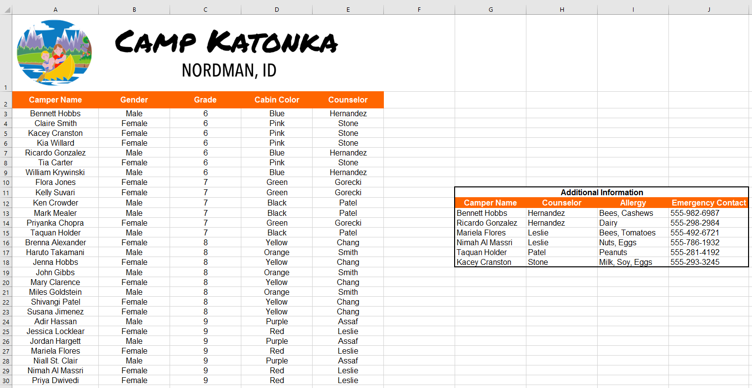
Lesson 20: Filtering Data
Introduction
If your worksheet contains a lot of content, it can be difficult to find information quickly. Filters can be used to narrow down the data in your worksheet, allowing you to view only the information you need.
Optional: Download our practice workbook.
Watch the video below to learn more about filtering data in Excel.
To filter data:
In our example, we'll apply a filter to an equipment log worksheet to display only the laptops and projectors that are available for checkout.
- In order for filtering to work correctly, your worksheet should include a header row, which is used to identify the name of each column. In our example, our worksheet is organized into different columns identified by the header cells in row 1: ID#, Type, Equipment Detail, and so on.
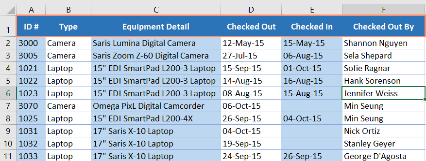
- Select the Data tab, then click the Filter command.
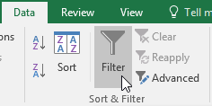
- A drop-down arrow will appear in the header cell for each column.
- Click the drop-down arrow for the column you want to filter. In our example, we will filter column B to view only certain types of equipment.
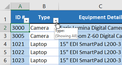
- The Filter menu will appear.
- Uncheck the box next to Select All to quickly deselect all data.
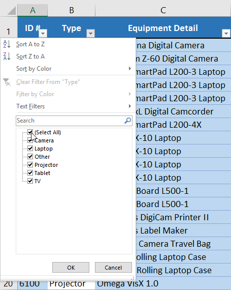
- Check the boxes next to the data you want to filter, then click OK. In this example, we will check Laptop and Projector to view only these types of equipment.
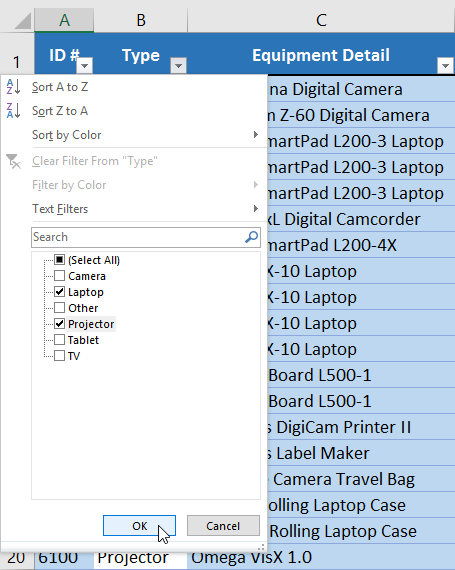
- The data will be filtered, temporarily hiding any content that doesn't match the criteria. In our example, only laptops and projectors are visible.
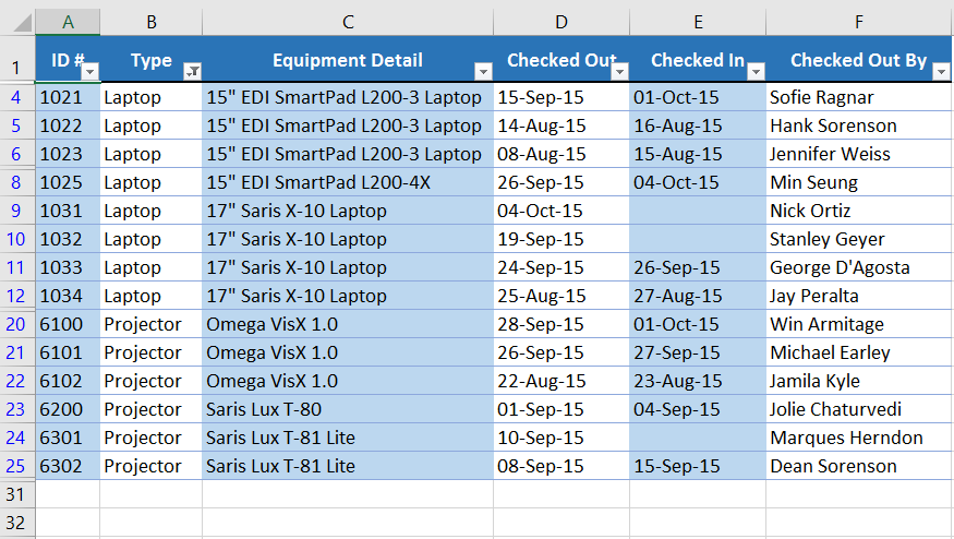
Filtering options can also be accessed from the Sort & Filter command on the Home tab.

To apply multiple filters:
Filters are cumulative, which means you can apply multiple filters to help narrow down your results. In this example, we've already filtered our worksheet to show laptops and projectors, and we'd like to narrow it down further to only show laptops and projectors that were checked out in August.
- Click the drop-down arrow for the column you want to filter. In this example, we will add a filter to column D to view information by date.
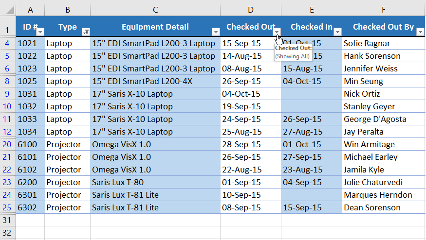
- The Filter menu will appear.
- Check or uncheck the boxes depending on the data you want to filter, then click OK. In our example, we'll uncheck everything except for August.
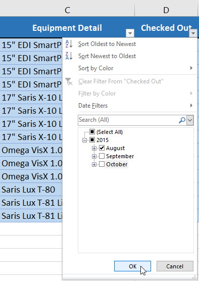
- The new filter will be applied. In our example, the worksheet is now filtered to show only laptops and projectors that were checked out in August.
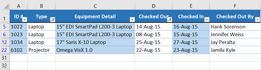
To clear a filter:
After applying a filter, you may want to remove—or clear—it from your worksheet so you'll be able to filter content in different ways.
- Click the drop-down arrow for the filter you want to clear. In our example, we'll clear the filter in column D.
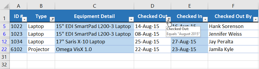
- The Filter menu will appear.
- Choose Clear Filter From [COLUMN NAME] from the Filter menu. In our example, we'll select Clear Filter From "Checked Out".
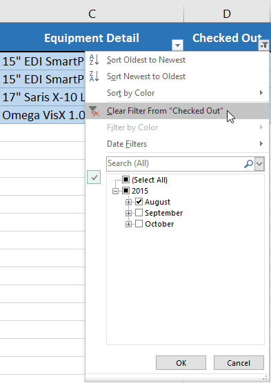
- The filter will be cleared from the column. The previously hidden data will be displayed.
To remove all filters from your worksheet, click the Filter command on the Data tab.
Advanced filtering
If you need a filter for something specific, basic filtering may not give you enough options. Fortunately, Excel includes many advanced filtering tools, including search, text, date, and number filtering, which can narrow your results to help find exactly what you need.
To filter with search:
Excel allows you to search for data that contains an exact phrase, number, date, and more. In our example, we'll use this feature to show only Saris brand products in our equipment log.
- Select the Data tab, then click the Filter command. A drop-down arrow will appear in the header cell for each column. Note: If you've already added filters to your worksheet, you can skip this step.
- Click the drop-down arrow for the column you want to filter. In our example, we'll filter column C.
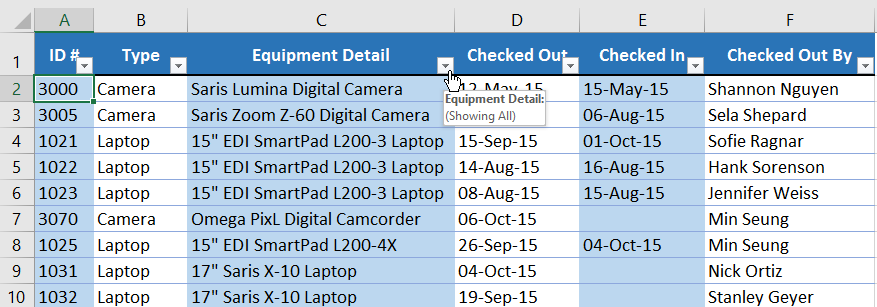
- The Filter menu will appear. Enter a search term into the search box. Search results will appear automatically below the Text Filters field as you type. In our example, we'll type saris to find all Saris brand equipment. When you're done, click OK.
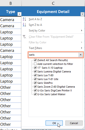
- The worksheet will be filtered according to your search term. In our example, the worksheet is now filtered to show only Saris brand equipment.
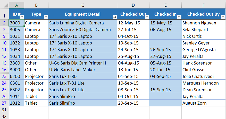
To use advanced text filters:
Advanced text filters can be used to display more specific information, like cells that contain a certain number of characters or data that excludes a specific word or number. In our example, we'd like to exclude any item containing the word laptop.
- Select the Data tab, then click the Filter command. A drop-down arrow will appear in the header cell for each column. Note: If you've already added filters to your worksheet, you can skip this step.
- Click the drop-down arrow for the column you want to filter. In our example, we'll filter column C.
- The Filter menu will appear. Hover the mouse over Text Filters, then select the desired text filter from the drop-down menu. In our example, we'll choose Does Not Contain to view data that does not contain specific text.
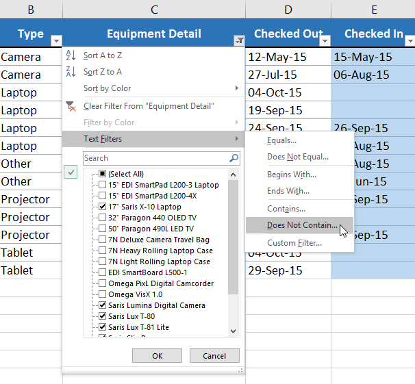
- The Custom AutoFilter dialog box will appear. Enter the desired text to the right of the filter, then click OK. In our example, we'll type laptop to exclude any items containing this word.
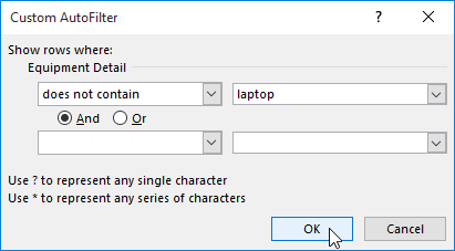
- The data will be filtered by the selected text filter. In our example, our worksheet now displays items that do not contain the word laptop.
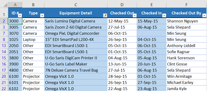
To use advanced number filters:
Advanced number filters allow you to manipulate numbered data in different ways. In this example, we'll display only certain types of equipment based on the range of ID numbers.
- Select the Data tab on the Ribbon, then click the Filter command. A drop-down arrow will appear in the header cell for each column. Note: If you've already added filters to your worksheet, you can skip this step.
- Click the drop-down arrow for the column you want to filter. In our example, we'll filter column A to view only a certain range of ID numbers.
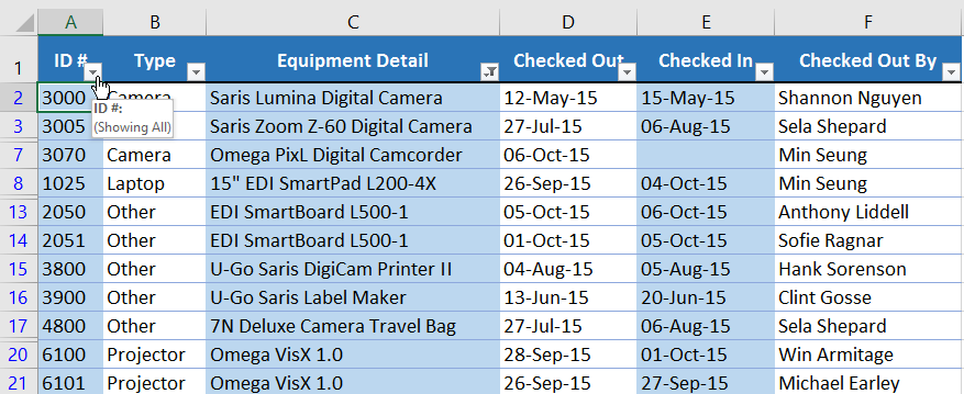
- The Filter menu will appear. Hover the mouse over Number Filters, then select the desired number filter from the drop-down menu. In our example, we'll choose Between to view ID numbers between a specific number range.
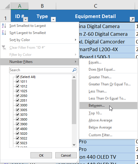
- The Custom AutoFilter dialog box will appear. Enter the desired number(s) to the right of each filter, then click OK. In our example, we want to filter for ID numbers greater than or equal to 3000 but less than or equal to 6000, which will display ID numbers in the 3000-6000 range.
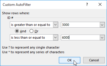
- The data will be filtered by the selected number filter. In our example, only items with an ID number between 3000 and 6000 are visible.
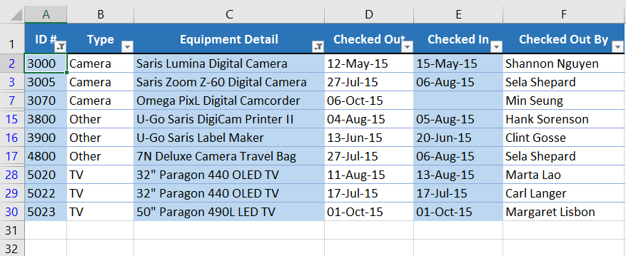
To use advanced date filters:
Advanced date filters can be used to view information from a certain time period, such as last year, next quarter, or between two dates. In this example, we'll use advanced date filters to view only equipment that has been checked out between July 15 and August 15.
- Select the Data tab, then click the Filter command. A drop-down arrow will appear in the header cell for each column. Note: If you've already added filters to your worksheet, you can skip this step.
- Click the drop-down arrow for the column you want to filter. In our example, we'll filter column D to view only a certain range of dates.
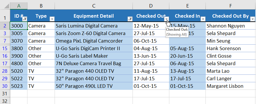
- The Filter menu will appear. Hover the mouse over Date Filters, then select the desired date filter from the drop-down menu. In our example, we'll select Between to view equipment that has been checked out between July 15 and August 15.
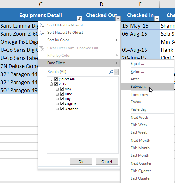
- The Custom AutoFilter dialog box will appear. Enter the desired date(s) to the right of each filter, then click OK. In our example, we want to filter for dates after or equal to July 15, 2015, and before or equal to August 15, 2015, which will display a range between these dates.
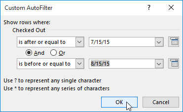
- The worksheet will be filtered by the selected date filter. In our example, we can now see which items have been checked out between July 15 and August 15.
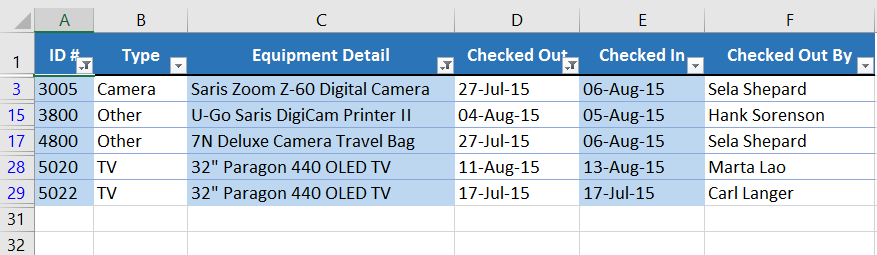
Challenge!
- Open our practice workbook.
- Click the Challenge tab in the bottom-left of the workbook.
- Apply a filter to show only Electronics and Instruments.
- Use the Search feature to filter item descriptions that contain the word Sansei. After you do this, you should have six entries showing.
- Clear the Item Description filter.
- Using a number filter, show loan amounts greater than or equal to $100.
- Filter to show only items that have deadlines in 2016.
- When you're finished, your workbook should look like this:
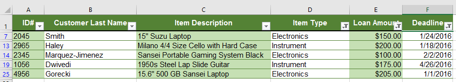
Lesson 21: Groups and Subtotals
Introduction
Worksheets with a lot of content can sometimes feel overwhelming and even become difficult to read. Fortunately, Excel can organize data into groups, allowing you to easily show and hide different sections of your worksheet. You can also summarize different groups using the Subtotal command and create an outline for your worksheet.
Optional: Download our practice workbook.
Watch the video below to learn more about groups and subtotals in Excel.
To group rows or columns:
- Select the rows or columns you want to group. In this example, we'll select columns B, C, and D.
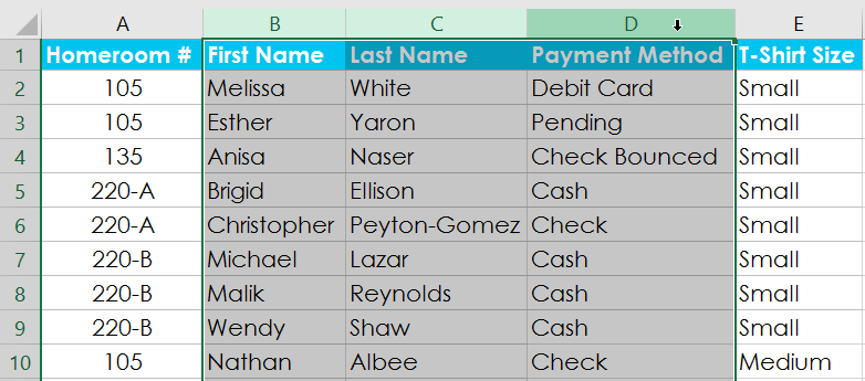
- Select the Data tab on the Ribbon, then click the Group command.
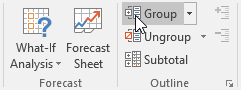
- The selected rows or columns will be grouped. In our example, columns B, C, and D are grouped.

To ungroup data, select the grouped rows or columns, then click the Ungroup command.
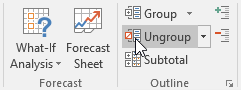
To hide and show groups:
- To hide a group, click the minus sign, also known as the Hide Detail button.
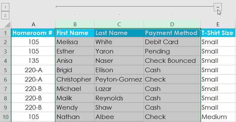
- The group will be hidden. To show a hidden group, click the plus sign, also known as the Show Detail button.
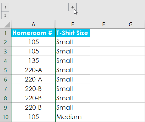
Creating subtotals
The Subtotal command allows you to automatically create groups and use common functions like SUM, COUNT, and AVERAGE to help summarize your data. For example, the Subtotal command could help to calculate the cost of office supplies by type from a large inventory order. It will create a hierarchy of groups, known as an outline, to help organize your worksheet.
Your data must be correctly sorted before using the Subtotal command, so you may want to review our lesson on Sorting Data to learn more.
To create a subtotal:
In our example, we'll use the Subtotal command with a T-shirt order form to determine how many T-shirts were ordered in each size (Small, Medium, Large, and X-Large). This will create an outline for our worksheet with a group for each T-shirt size and then count the total number of shirts in each group.
- First, sort your worksheet by the data you want to subtotal. In this example, we'll create a subtotal for each T-shirt size, so our worksheet has been sorted by T-shirt size from smallest to largest.
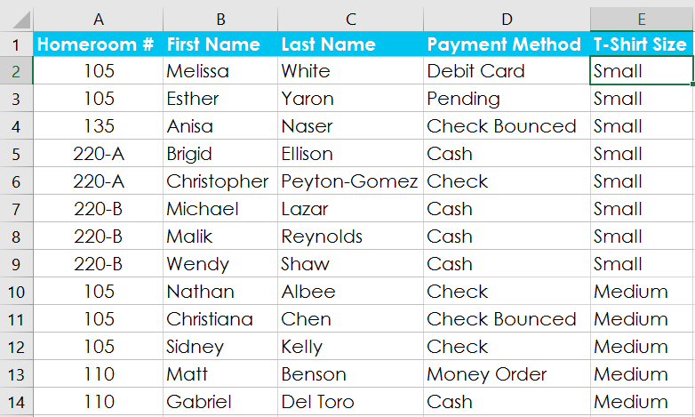
- Select the Data tab, then click the Subtotal command.
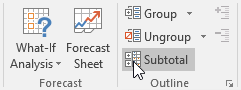
- The Subtotal dialog box will appear. Click the drop-down arrow for the At each change in: field to select the column you want to subtotal. In our example, we'll select T-Shirt Size.
- Click the drop-down arrow for the Use function: field to select the function you want to use. In our example, we'll select COUNT to count the number of shirts ordered in each size.
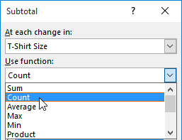
- In the Add subtotal to: field, select the column where you want the calculated subtotal to appear. In our example, we'll select T-Shirt Size. When you're satisfied with your selections, click OK.
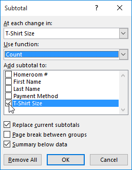
- The worksheet will be outlined into groups, and the subtotal will be listed below each group. In our example, the data is now grouped by T-shirt size, and the number of shirts ordered in that size appears below each group.
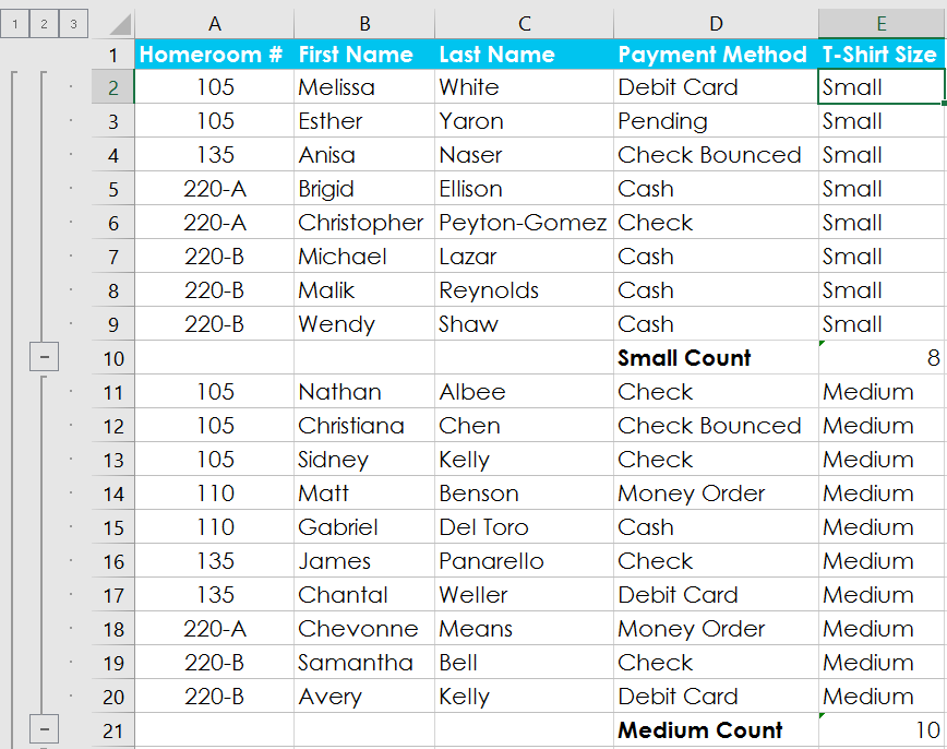
To view groups by level:
When you create subtotals, your worksheet it is divided into different levels. You can switch between these levels to quickly control how much information is displayed in the worksheet by clicking the Level buttons to the left of the worksheet. In our example, we'll switch between all three levels in our outline. While this example contains only three levels, Excel can accommodate up to eight.
- Click the lowest level to display the least detail. In our example, we'll select level 1, which contains only the grand count, or total number of T-shirts ordered.
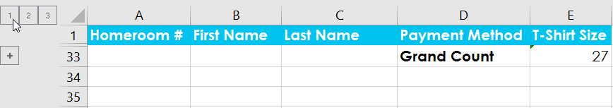
- Click the next level to expand the detail. In our example, we'll select level 2, which contains each subtotal row but hides all other data from the worksheet.
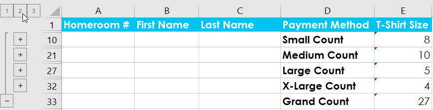
- Click the highest level to view and expand all of your worksheet data. In our example, we'll select level 3.
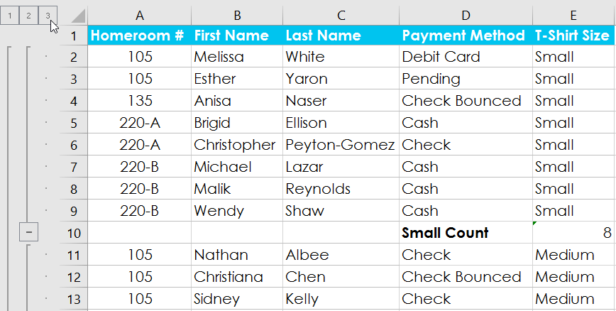
You can also use the Show and Hide Detail buttons to show and hide the groups within the outline.
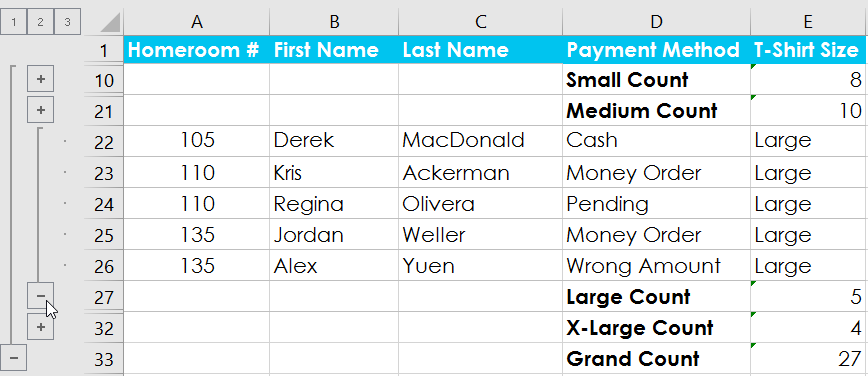
To remove subtotals:
Sometimes you may not want to keep subtotals in your worksheet, especially if you want to reorganize data in different ways. If you no longer want to use subtotaling, you'll need remove it from your worksheet.
- Select the Data tab, then click the Subtotal command.
- The Subtotal dialog box will appear. Click Remove All.
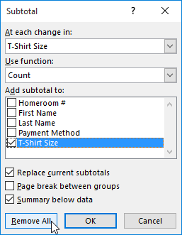
- All worksheet data will be ungrouped, and the subtotals will be removed.
To remove all groups without deleting the subtotals, click the Ungroup command drop-down arrow, then choose Clear Outline.
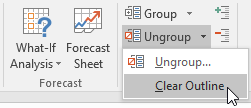
Challenge!
- Open our practice workbook.
- Click on the Challenge tab in the bottom-left of the workbook.
- Sort the workbook by Grade from smallest to largest.
- Use the Subtotal command to group at each change in Grade. Use the SUM function and add subtotals to Amount Raised.
- Select Level 2 so that you only see the subtotals and grand total.
- When you're finished, your workbook should look like this:
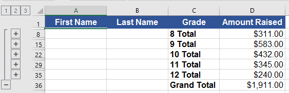
Lesson 22: Tables
Introduction
Once you've entered information into your worksheet, you may want to format your data as a table. Just like regular formatting, tables can improve the look and feel of your workbook, and they'll also help you organize your content and make your data easier to use. Excel includes several tools and predefined table styles, allowing you to create tables quickly and easily.
Optional: Download our practice workbook.
Watch the video below to learn more about working with tables.
To format data as a table:
- Select the cells you want to format as a table. In our example, we'll select the cell range A2:D9.
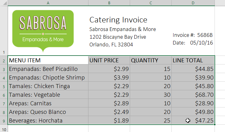
- From the Home tab, click the Format as Table command in the Styles group.
- Select a table style from the drop-down menu.
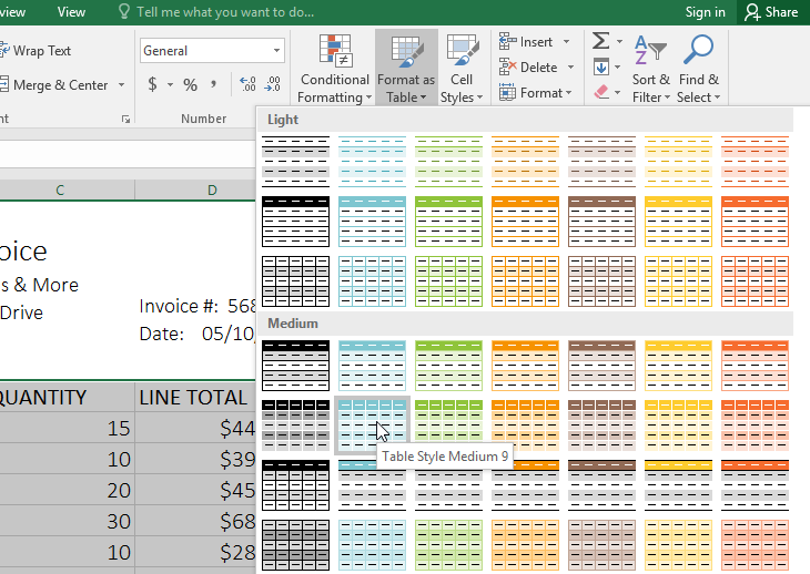
- A dialog box will appear, confirming the selected cell range for the table.
- If your table has headers, check the box next to My table has headers, then click OK.
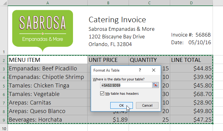
- The cell range will be formatted in the selected table style.
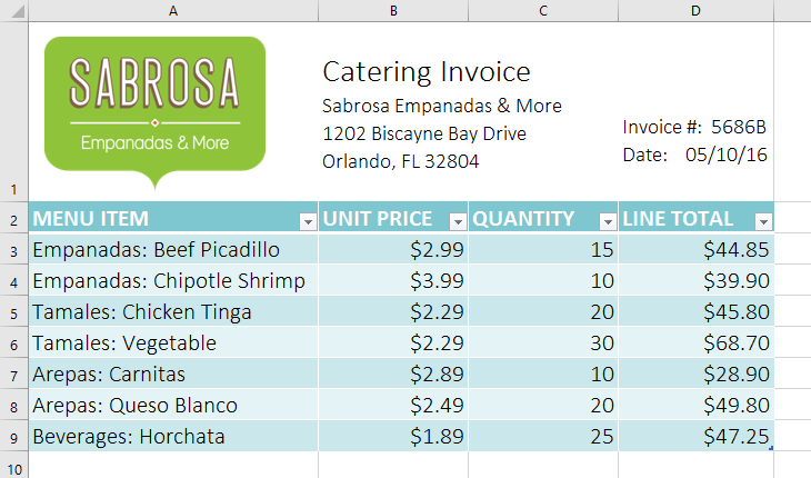
Tables include filtering by default. You can filter your data at any time using the drop-down arrows in the header cells. To learn more, review our lesson on Filtering Data.
Modifying tables
It's easy to modify the look and feel of any table after adding it to a worksheet. Excel includes many different options for customizing a table, including adding rows or columns and changing the table style.
To add rows or columns to a table:
If you need to fit more content into your table, Excel allows you to modify the table size by including additional rows and columns. There are two simple ways to change the table size:
- Enter new content into any adjacent row or column. The row or column will be roped into the table automatically.
- Click and drag the bottom-right corner of the table to create additional rows or columns.
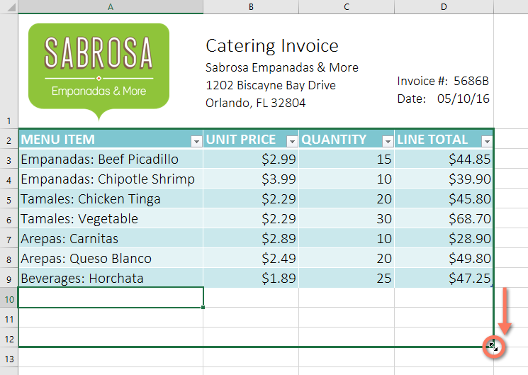
To change the table style:
- Select any cell in your table, then click the Design tab.
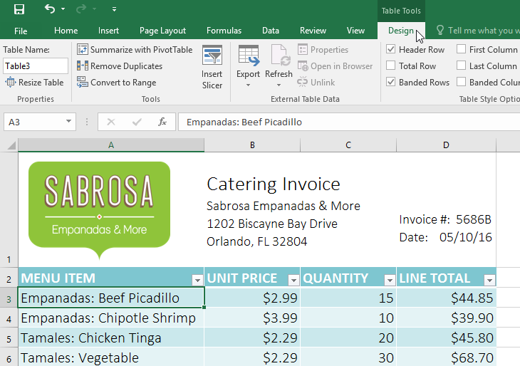
- Locate the Table Styles group, then click the More drop-down arrow to see all available table styles.
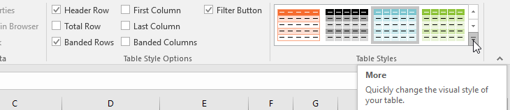
- Select the desired table style.
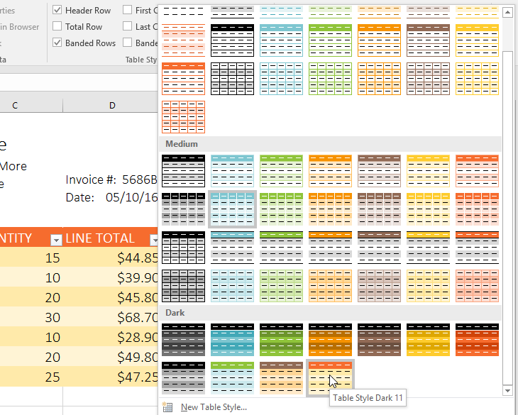
- The table style will be applied.
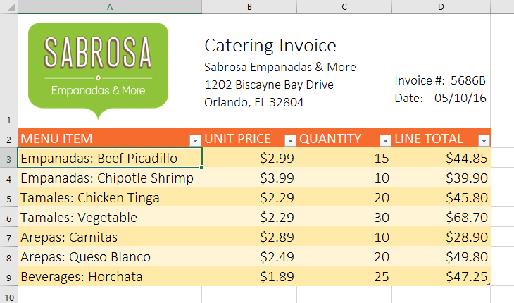
To modify table style options:
You can turn various options on or off to change the appearance of any table. There are several options: Header Row, Total Row, Banded Rows, First Column, Last Column, Banded Columns, and Filter Button.Select any cell in your table, then click the Design tab.
- Check or uncheck the desired options in the Table Style Options group. In our example, we'll check Total Row to automatically include a total for our table.
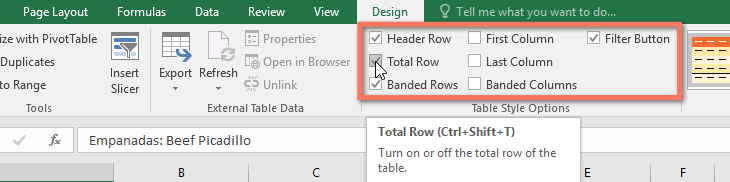
- The table style will be modified. In our example, a new row has been added to the table with a formula that automatically calculates the total value of the cells in column D.
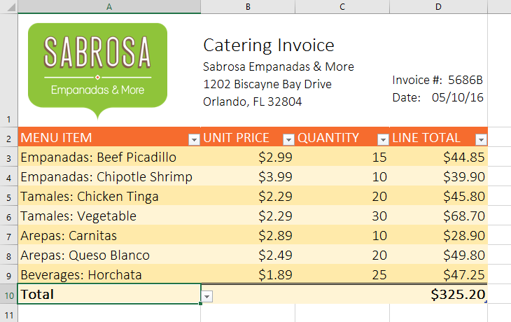
Depending on the type of content you have—and the table style you've chosen—these options can affect your table's appearance in various ways. You may need to experiment with a few different options to find the exact style you want.
To remove a table:
It's possible to remove a table from your workbook without losing any of your data. However, this can cause issues with certain types of formatting, including colors, fonts, and banded rows. Before you use this option, make sure you're prepared to reformat your cells if necessary.
- Select any cell in your table, then click the Design tab.
- Click the Convert to Range command in the Tools group.
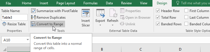
- A dialog box will appear. Click Yes.
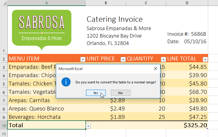
- The range will no longer be a table, but the cells will retain their data and formatting.
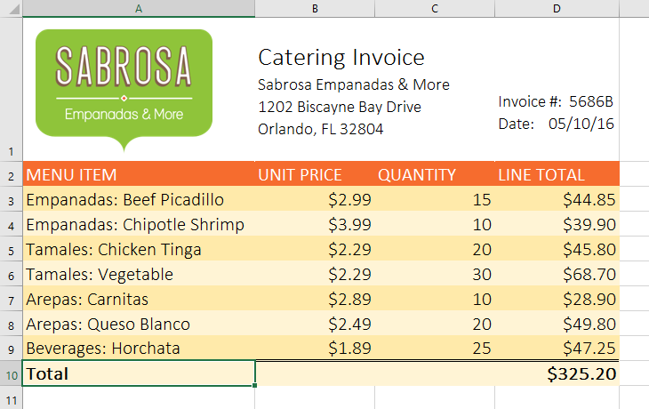
To restart your formatting from scratch, click the Clear command on the Home tab. Next, choose Clear Formats from the menu.
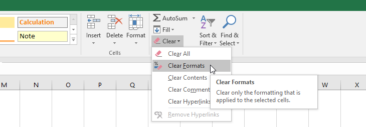
Challenge!
- Open our practice workbook.
- Click the Challenge tab in the bottom-left of the workbook.
- Select cells A2:D9 and format as table. Choose one of the light styles.
- Insert a row between rows 4 and 5. In the row you just created, type Empanadas: Banana and Nutella, with a unit price of $3.25, and a quantity of 12.
- Change the table style to Table Style Medium 10.
- In Table Style Options, uncheck banded rows and check banded columns.
- When you're finished, your workbook should look like this:
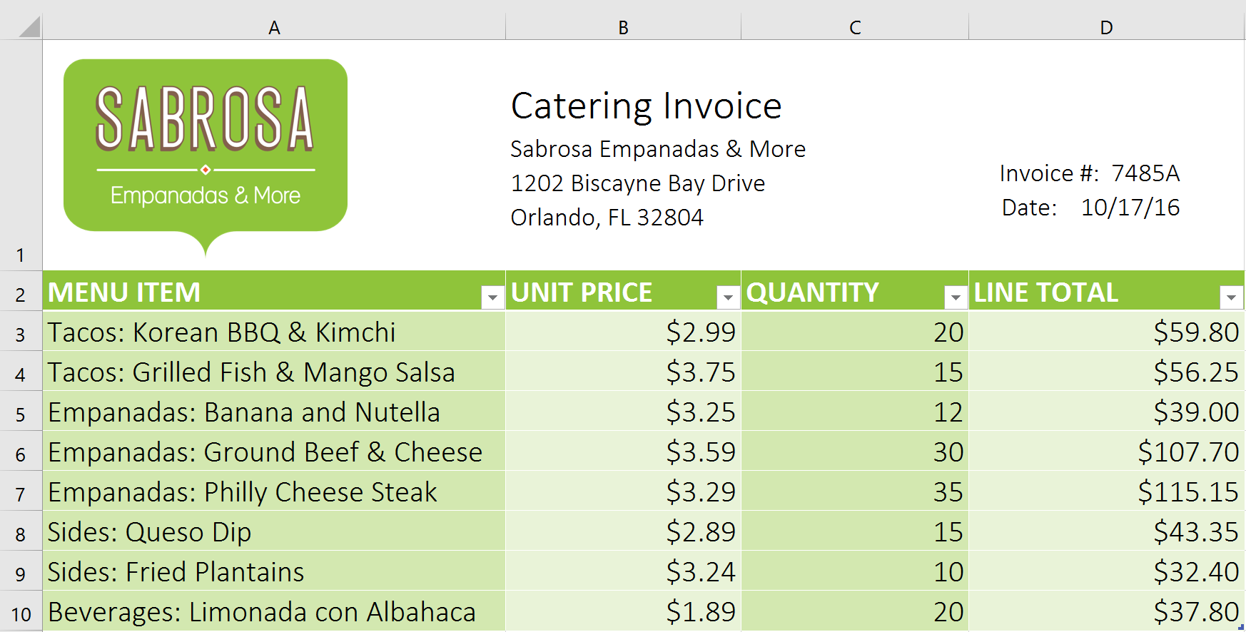
Lesson 23: Charts
Introduction
It can be difficult to interpret Excel workbooks that contain a lot of data. Charts allow you to illustrate your workbook data graphically, which makes it easy to visualize comparisons and trends.
Optional: Download our practice workbook.
Watch the video below to learn more about charts.
Understanding charts
Excel has several different types of charts, allowing you to choose the one that best fits your data. In order to use charts effectively, you'll need to understand how different charts are used.
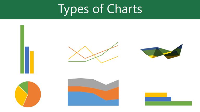
Excel has a variety of chart types, each with its own advantages. Click the arrows to see some of the different types of charts available in Excel.
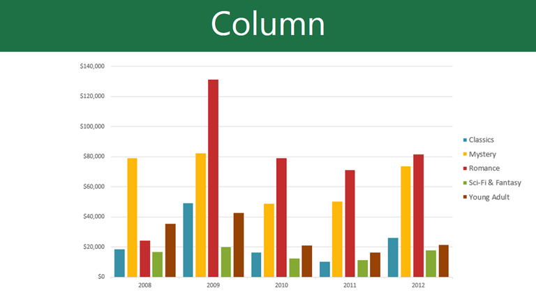
Column charts use vertical bars to represent data. They can work with many different types of data, but they're most frequently used for comparing information.
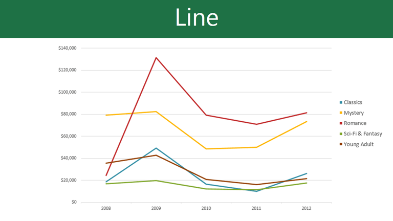
Line charts are ideal for showing trends. The data points are connected with lines, making it easy to see whether values are increasing or decreasing over time.
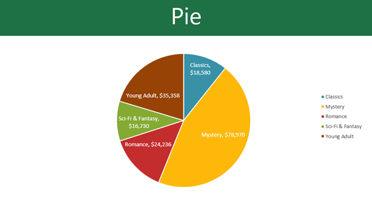
Pie charts make it easy to compare proportions. Each value is shown as a slice of the pie, so it's easy to see which values make up the percentage of a whole.
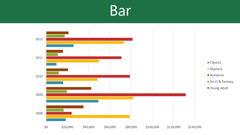
Bar charts work just like column charts, but they use horizontal rather than vertical bars.
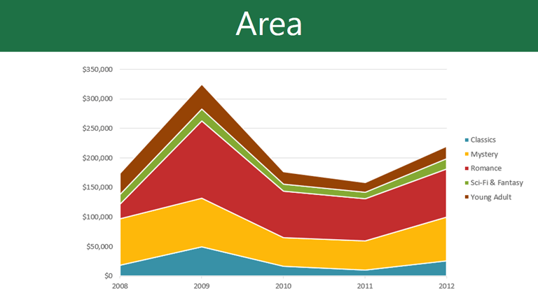
Area charts are similar to line charts, except the areas under the lines are filled in.
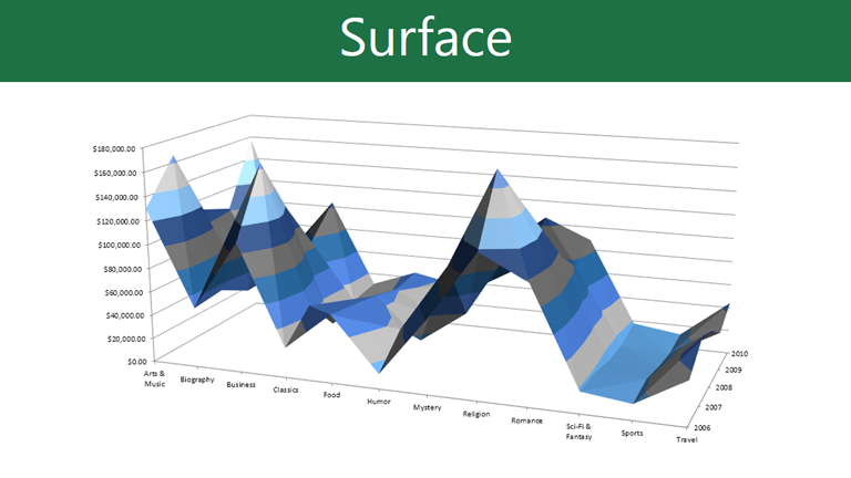
Surface charts allow you to display data across a 3D landscape. They work best with large data sets, allowing you to see a variety of information at the same time.

In addition to chart types, you'll need to understand how to read a chart. Charts contain several different elements, or parts, that can help you interpret the data.
Click the buttons in the interactive below to learn about the different parts of a chart.
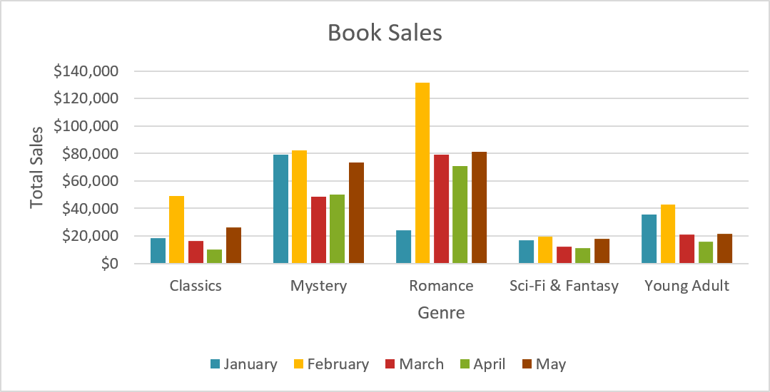
To insert a chart:
- Select the cells you want to chart, including the column titles and row labels. These cells will be the source data for the chart. In our example, we'll select cells A1:F6.
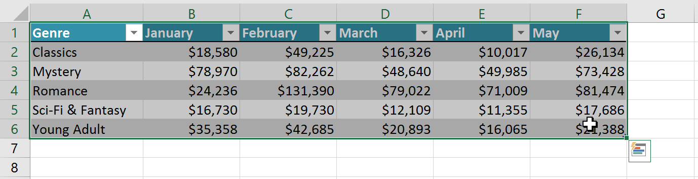
- From the Insert tab, click the desired Chart command. In our example, we'll select Column.
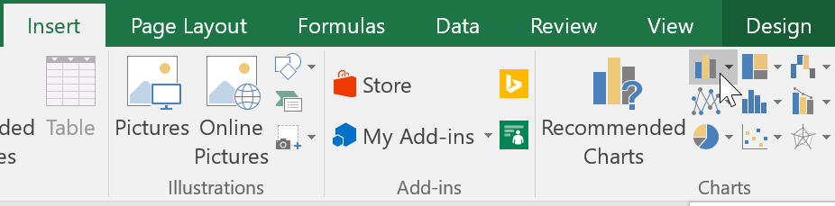
- Choose the desired chart type from the drop-down menu.
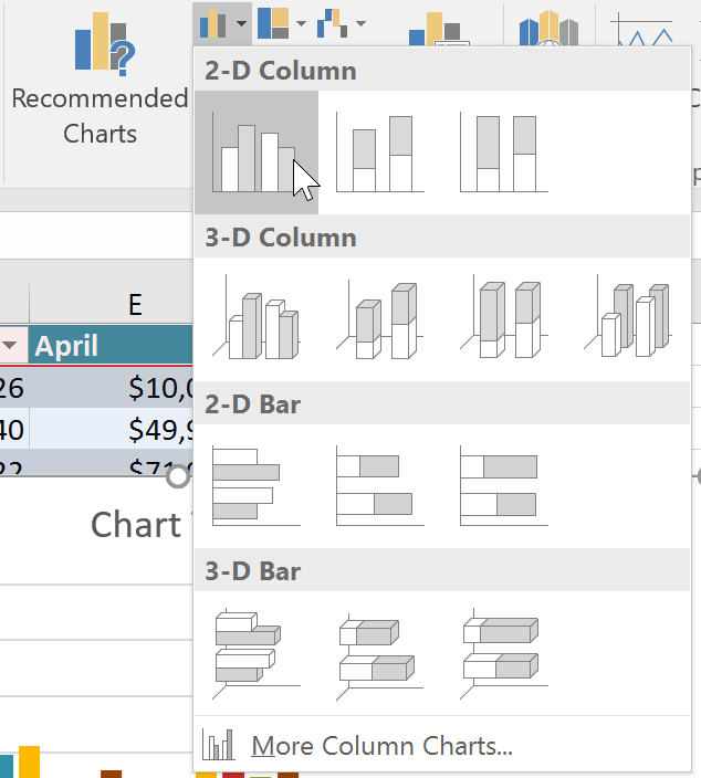
- The Selected chart will be inserted into the worksheet.

If you're not sure which type of chart to use, the Recommended Charts command will suggest several different charts based on the source data.
Chart and layout style
After inserting a chart, there are several things you may want to change about the way your data is displayed. It's easy to edit a chart's layout and style from the Design tab.
- Excel allows you to add chart elements—such as chart titles, legends, and data labels—to make your chart easier to read. To add a chart element, click the Add Chart Element command on the Design tab, then choose the desired element from the drop-down menu.
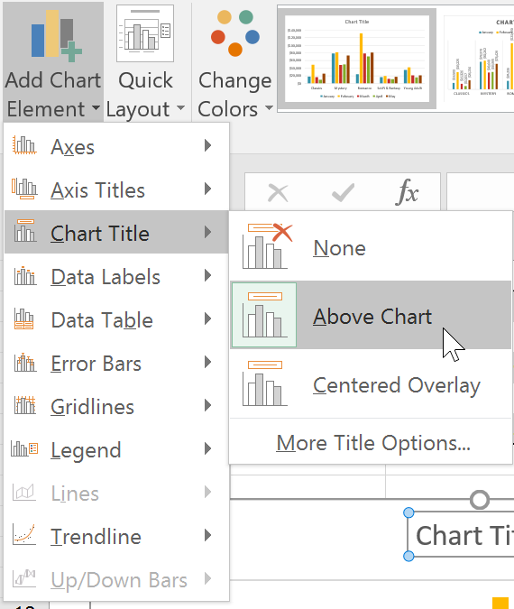
- To edit a chart element, like a chart title, simply double-click the placeholder and begin typing.
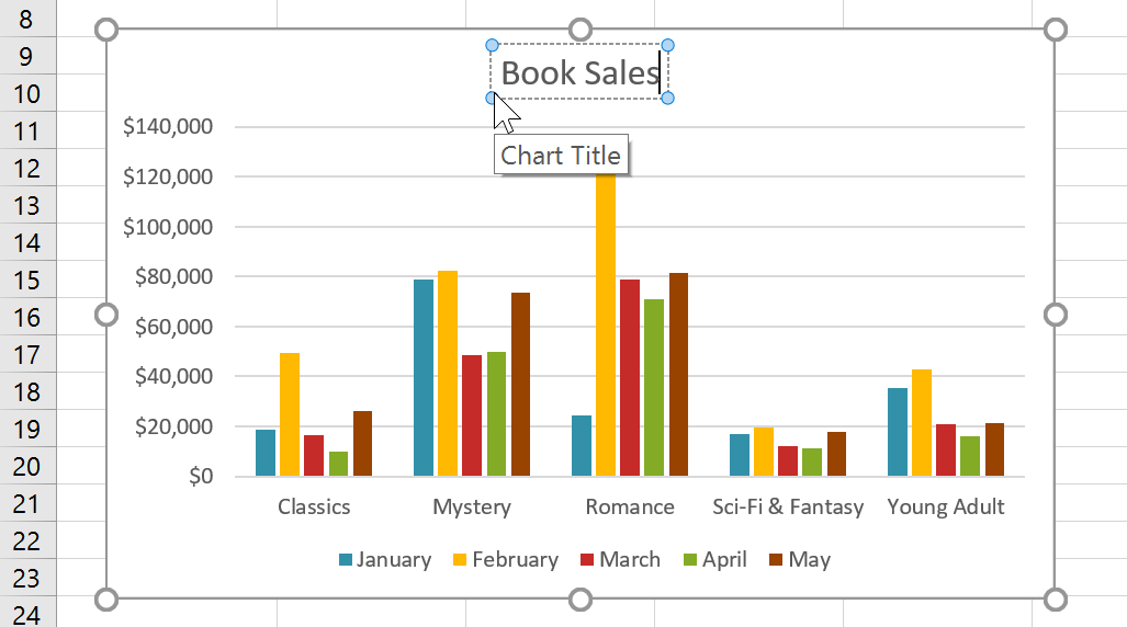
- If you don't want to add chart elements individually, you can use one of Excel's predefined layouts. Simply click the Quick Layout command, then choose the desired layout from the drop-down menu.
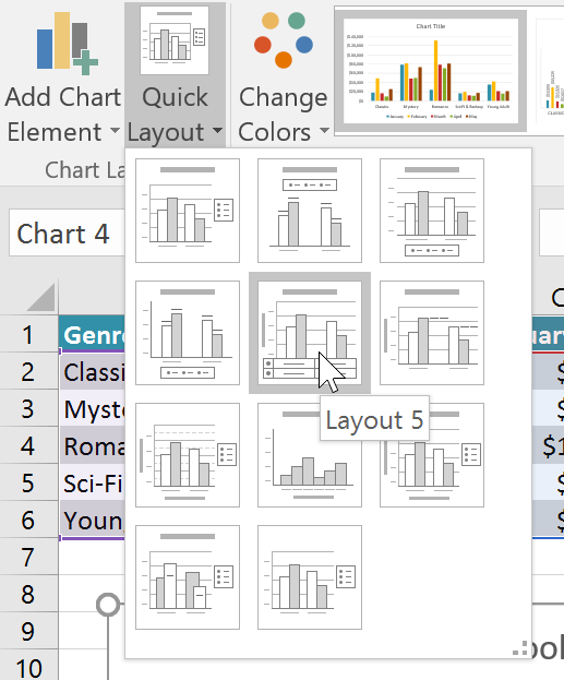
- Excel also includes several chart styles, which allow you to quickly modify the look and feel of your chart. To change the chart style, select the desired style from the Chart styles group. You can also click the drop-down arrow on the right to see more styles.
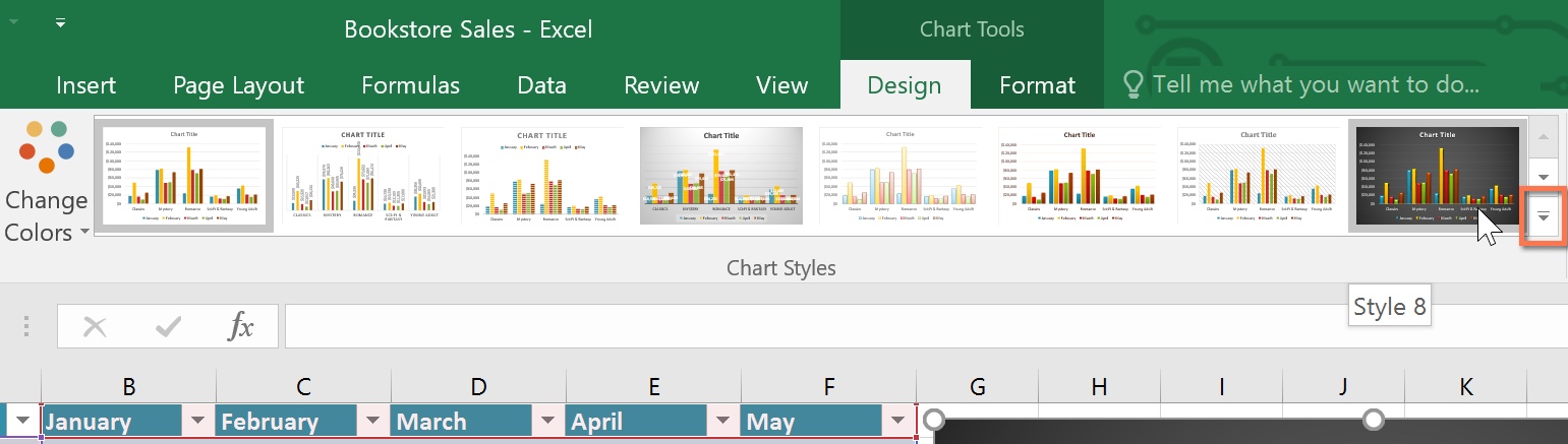
You can also use the chart formatting shortcut buttons to quickly add chart elements, change the chart style, and filter the chart data.
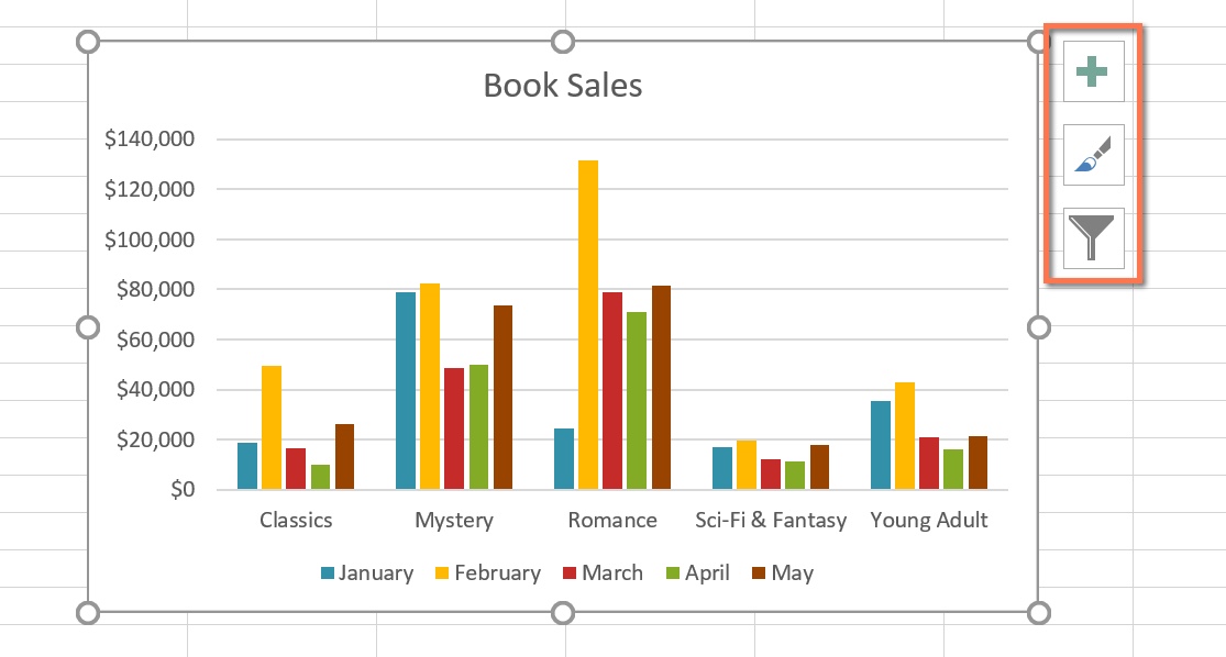
Other chart options
There are many other ways to customize and organize your charts. For example, Excel allows you to rearrange a chart's data, change the chart type, and even move the chart to a different location in a workbook.
To switch row and column data:
Sometimes you may want to change the way charts group your data. For example, in the chart below Book Sales data is grouped by genre, with columns for each month. However, we could switch the rows and columns so the chart will group the data by month, with columns for each genre. In both cases, the chart contains the same data—it's just organized differently.
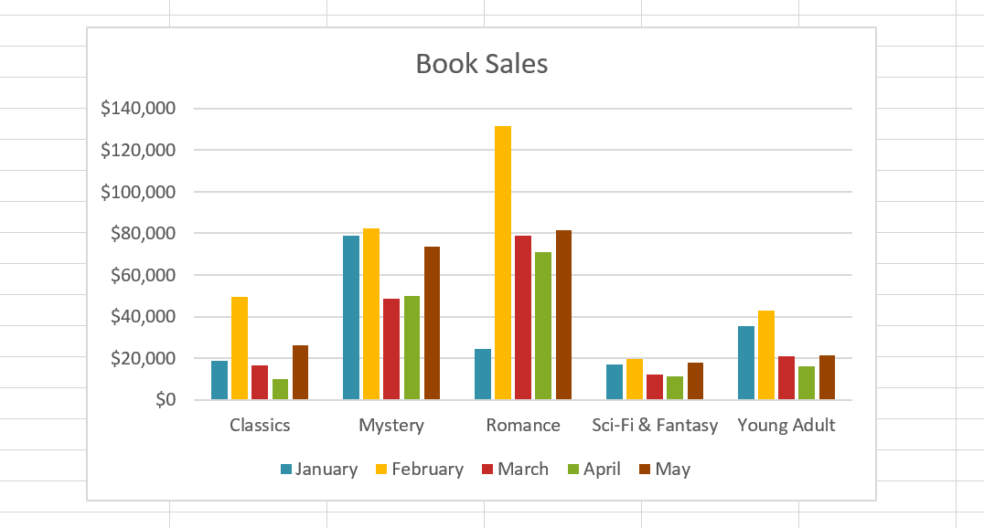
- Select the chart you want to modify.
- From the Design tab, select the Switch Row/Column command.
- The rows and columns will be switched. In our example, the data is now grouped by month, with columns for each genre.
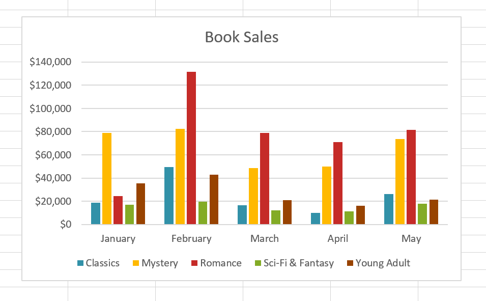
To change the chart type:
If you find that your data isn't well suited to a certain chart, it's easy to switch to a new chart type. In our example, we'll change our chart from a column chart to a line chart.
- From the Design tab, click the Change Chart Type command.
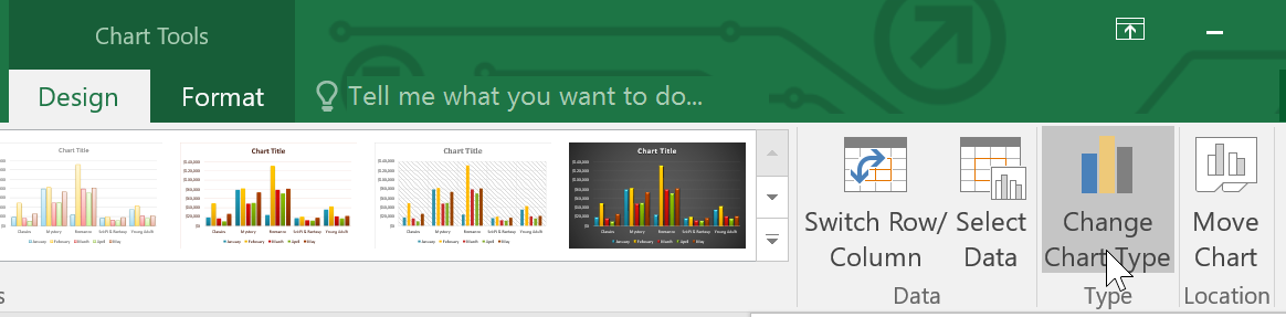
- The Change Chart Type dialog box will appear. Select a new chart type and layout, then click OK. In our example, we'll choose a Line chart.
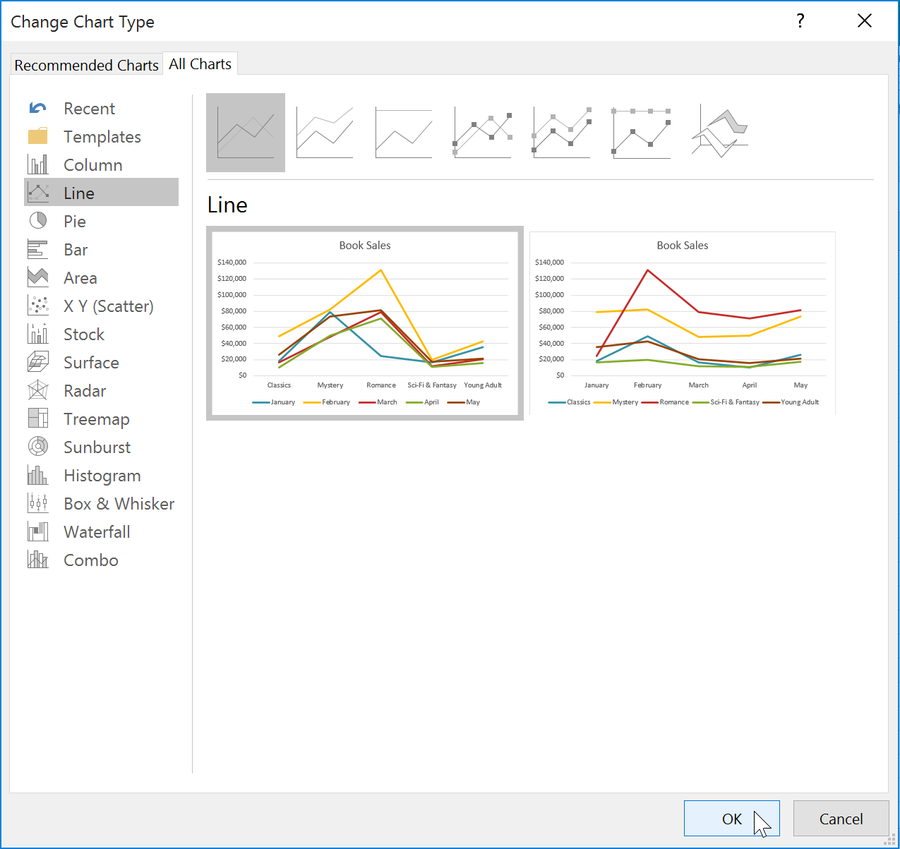
- The selected chart type will appear. In our example, the line chart makes it easier to see trends in sales data over time.
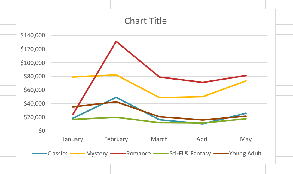
To move a chart:
Whenever you insert a new chart, it will appear as an object on the same worksheet that contains its source data. Alternatively, you can move the chart to a new worksheet to help keep your data organized.
- Select the chart you want to move.
- Click the Design tab, then select the Move Chart command.
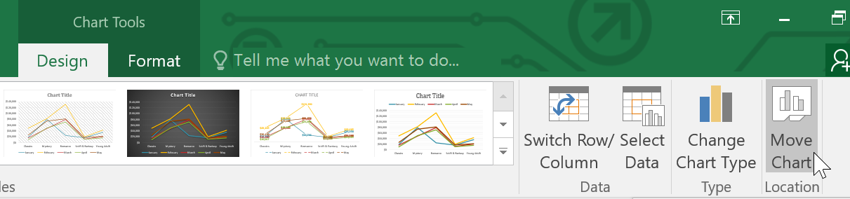
- The Move Chart dialog box will appear. Select the desired location for the chart. In our example, we'll choose to move it to a New sheet, which will create a new worksheet.
- Click OK.
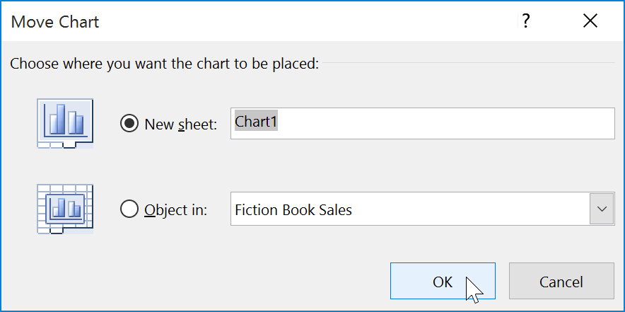
- The chart will appear in the selected location. In our example, the chart now appears on a new worksheet.
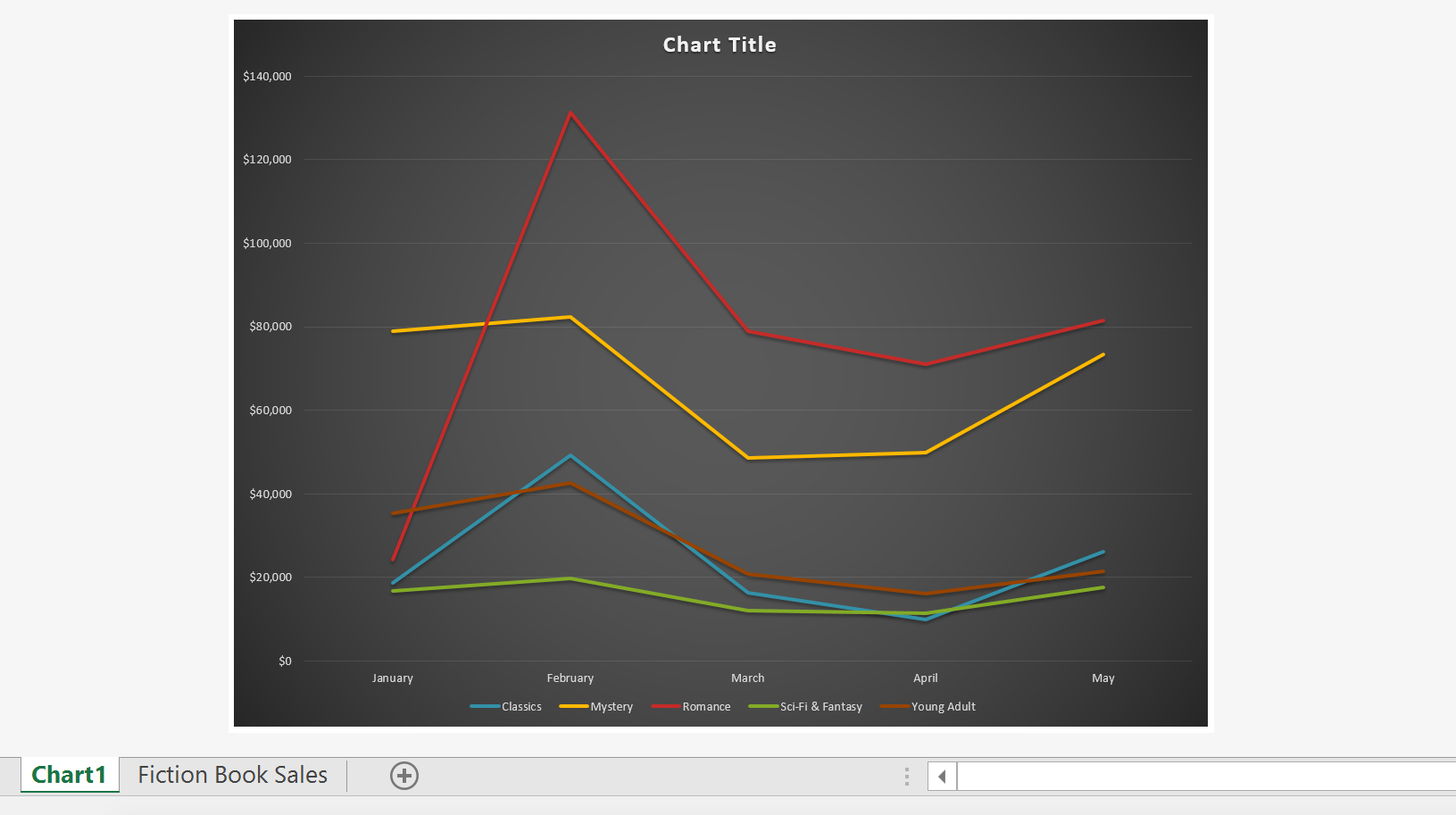
Keeping charts up to date
By default, when you add more data to your spreadsheet, the chart may not include the new data. To fix this, you can adjust the data range. Simply click the chart, and it will highlight the data range in your spreadsheet. You can then click and drag the handle in the lower-right corner to change the data range.
If you frequently add more data to your spreadsheet, it may become tedious to update the data range. Luckily, there is an easier way. Simply format your source data as a table, then create a chart based on that table. When you add more data below the table, it will automatically be included in both the table and the chart, keeping everything consistent and up to date.
Watch the video below to learn how to use tables to keep charts up to date.
Challenge!
- Open our practice workbook.
- Click the Challenge tab in the bottom-left of the workbook.
- Select cells A1:E6 and insert a 2D Clustered Column chart.
- Change the chart title to September to December Sales.
- Use the Switch Row/Column command. The columns should now be grouped by month, with a different color for each salesperson.
- Move the chart to a new sheet.
- Change the chart type to line with markers.
- Use the Quick Layout command to change the layout of the chart.
- When you're finished, your workbook should look something like this:
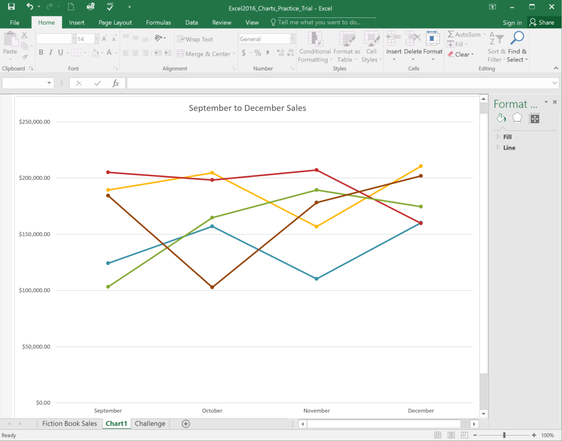
Lesson 24: Conditional Formatting
Introduction
Let's say you have a worksheet with thousands of rows of data. It would be extremely difficult to see patterns and trends just from examining the raw information. Similar to charts and sparklines, conditional formatting provides another way to visualize data and make worksheets easier to understand.
Optional: Download our practice workbook.
Watch the video below to learn more about conditional formatting in Excel.
Understanding conditional formatting
Conditional formatting allows you to automatically apply formatting—such as colors, icons, and data bars—to one or more cells based on the cell value. To do this, you'll need to create a conditional formatting rule. For example, a conditional formatting rule might be: If the value is less than $2000, color the cell red. By applying this rule, you'd be able to quickly see which cells contain values less than $2000.
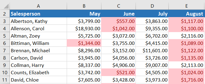
To create a conditional formatting rule:
In our example, we have a worksheet containing sales data, and we'd like to see which salespeople are meeting their monthly sales goals. The sales goal is $4000 per month, so we'll create a conditional formatting rule for any cells containing a value higher than 4000.
- Select the desired cells for the conditional formatting rule.
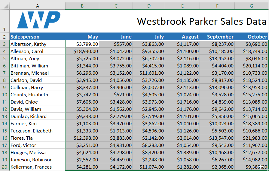
- From the Home tab, click the Conditional Formatting command. A drop-down menu will appear.
- Hover the mouse over the desired conditional formatting type, then select the desired rule from the menu that appears. In our example, we want to highlight cells that are greater than $4000.
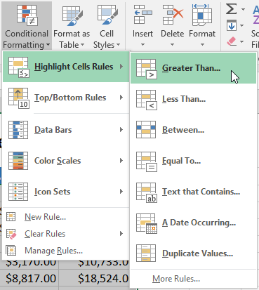
- A dialog box will appear. Enter the desired value(s) into the blank field. In our example, we'll enter 4000 as our value.
- Select a formatting style from the drop-down menu. In our example, we'll choose Green Fill with Dark Green Text, then click OK.
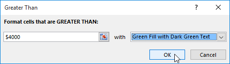
- The conditional formatting will be applied to the selected cells. In our example, it's easy to see which salespeople reached the $4000 sales goal for each month.
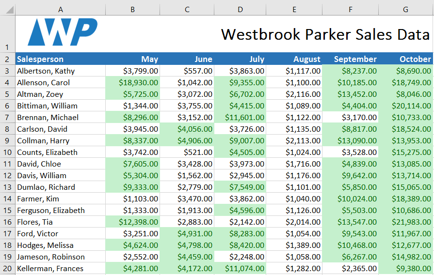
You can apply multiple conditional formatting rules to a cell range or worksheet, allowing you to visualize different trends and patterns in your data.
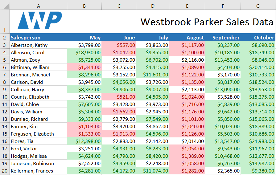
Conditional formatting presets
Excel has several predefined styles—or presets—you can use to quickly apply conditional formatting to your data. They are grouped into three categories:
- Data Bars are horizontal bars added to each cell, much like a bar graph.
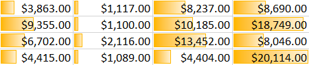
- Color Scales change the color of each cell based on its value. Each color scale uses a two- or three-color gradient. For example, in the Green-Yellow-Red color scale, the highest values are green, the average values are yellow, and the lowest values are red.
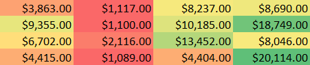
- Icon Sets add a specific icon to each cell based on its value.
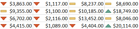
To use preset conditional formatting:
- Select the desired cells for the conditional formatting rule.
- Click the Conditional Formatting command. A drop-down menu will appear.
- Hover the mouse over the desired preset, then choose a preset style from the menu that appears.
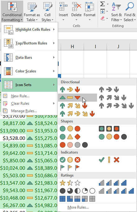
- The conditional formatting will be applied to the selected cells.

Removing conditional formatting
To remove conditional formatting:
- Click the Conditional Formatting command. A drop-down menu will appear.
- Hover the mouse over Clear Rules, and choose which rules you want to clear. In our example, we'll select Clear Rules from Entire Sheet to remove all conditional formatting from the worksheet.
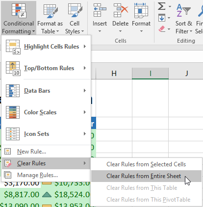
- The conditional formatting will be removed.
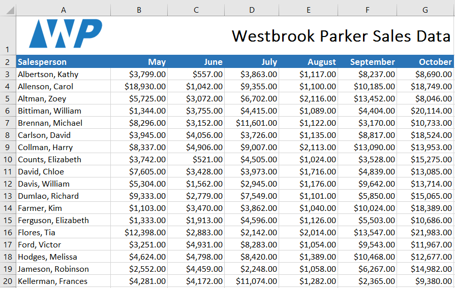
Click Manage Rules to edit or delete individual rules. This is especially useful if you've applied multiple rules to a worksheet.
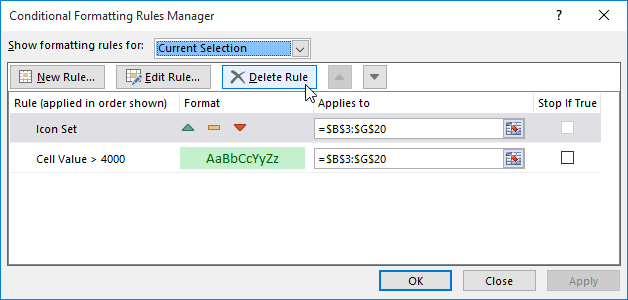
Challenge!
- Open our practice workbook.
- Click the Challenge worksheet tab in the bottom-left of the workbook.
- Select cells B3:J17.
- Let's say you're the teacher and want to easily see all of the grades that are below passing. Apply Conditional Formatting so it Highlights Cells containing values Less Than 70 with a light red fill.
- Now you want to see how the grades compare to each other. Under the Conditional Formatting tab, select the Icon Set called 3 Symbols (Circled). Hint: The names of the icon sets will appear when you hover over them.
- Your spreadsheet should look like this:
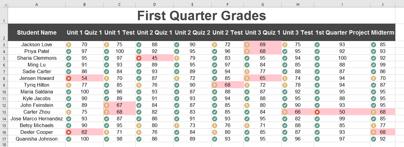
- Using the Manage Rules feature, remove the light red fill, but keep the icon set.
Lesson 25: Track Changes and Comments
Introduction
Let's say someone asked you to proofread or collaborate on a workbook. If you had a printed copy, you might use a red pen to edit cell data, mark spelling errors, or add comments in the margins. Excel allows you to do all of these things electronically using the Track Changes and Comments features.
Alert! The Track Changes command has been removed from the Review Tab in Excel 2016.
Optional: Download our practice workbook.
Watch the video below to learn more about track changes and comments.
Understanding Track Changes
When you turn on the Track Changes feature, every cell you edit will be highlighted with a unique border and indicator. Selecting a marked cell will show the details of the change. This allows you and other reviewers to see what's been changed before accepting the revisions permanently.
In the image below, each edited cell has a blue border and a small triangle in the upper-left corner.
There are some changes Excel cannot track. Before using this feature, you may want to review Microsoft's list of changes that Excel does not track or highlight.
You cannot use Track Changes if your workbook includes tables. To remove a table, select it, click the Design tab, then click Convert to Range.
To turn on Track Changes:
- From the Review tab, click the Track Changes command, then select Highlight Changes from the drop-down menu.
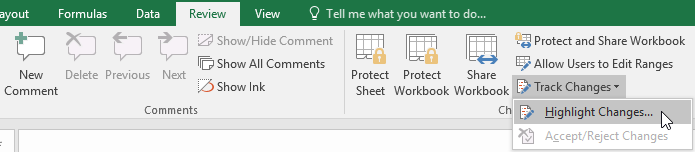
- The Highlight Changes dialog box will appear. Check the box next to Track changes while editing. Verify that the box is checked for Highlight changes on screen, then click OK.
- If prompted, click OK to allow Excel to save your workbook.
- Track Changes will be turned on. A triangle and border color will appear in any cell you edit. If there are multiple reviewers, each person will be assigned a different color.
- Select the edited cell to see a summary of the tracked changes. In our example below, we've changed the content of cell D14 from ? to Getting to know your team.
When you turn on Track Changes, your workbook will be shared automatically. Shared workbooks are designed to be stored where other users can access and edit the workbook at the same time, such as a network. However, you can also track changes in a local or personal copy, as seen throughout this lesson.
To list changes on a separate worksheet:
You can also view changes on a new worksheet, sometimes called the Tracked Changes history. The history lists everything in your worksheet that has been changed, including the old value (previous cell content) and the new value (current cell content).
- Save your workbook.
- From the Review tab, click the Track Changes command, then select Highlight Changes from the drop-down menu.
- The Highlight Changes dialog box will appear. Check the box next to List changes on a new sheet, then click OK.
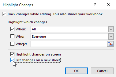
- The tracked changes will be listed on their own worksheet, called History.
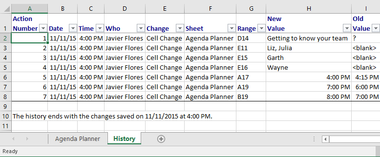
To remove the History worksheet from your workbook, you can either save your workbook again or uncheck the box next to List changes on a new sheet in the Highlight Changes dialog box.
Reviewing changes
Tracked changes are really just suggested changes. To become permanent, the changes must be accepted. On the other hand, the original author may disagree with some of the tracked changes and choose to reject them.
To review tracked changes:
- From the Review tab, click Track Changes, then select Accept/Reject Changes from the drop-down menu.
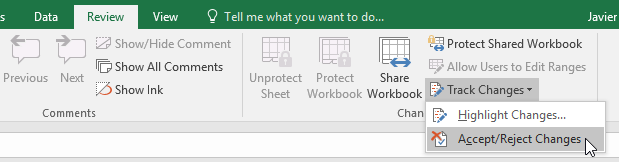
- If prompted, click OK to save your workbook.
- A dialog box will appear. Make sure the box next to the When: field is checked and set to Not yet reviewed, then click OK.
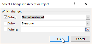
- A dialog box will appear. Click Accept or Reject for each change in the workbook. Excel will move through each change automatically until you have reviewed them all.
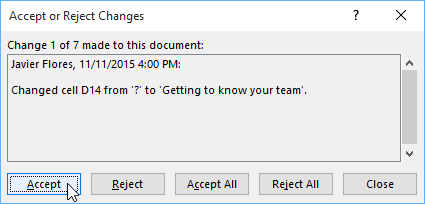
- Even after accepting or rejecting changes, the tracked changes will still appear in your workbook. To remove them completely, you'll need to turn off Track Changes. From the Review tab, click Track Changes, then select Highlight Changes from the drop-down menu.
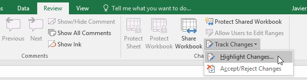
- A dialog box will appear. Uncheck the box next to Track changes while editing, then click OK.
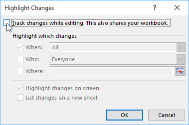
- Click Yes to confirm that you want to turn off Track Changes and stop sharing your workbook.
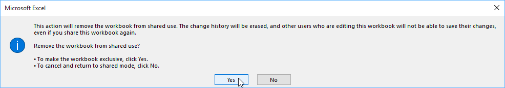
To accept or reject all changes at once, click Accept All or Reject All in the Accept or Reject Changes dialog box.
Turning off Track Changes will remove any tracked changes in your workbook. You will not be able to view, accept, or reject changes; instead, all changes will be accepted automatically. Always review the changes in your worksheet before turning off Track Changes.
Comments
Sometimes you may want to add a comment to provide feedback instead of editing the contents of a cell. While often used in combination with Track Changes, you don't necessarily need to have Track Changes turned on to use comments.
To add a comment:
- Select the cell where you want the comment to appear. In our example, we'll select cell D17.
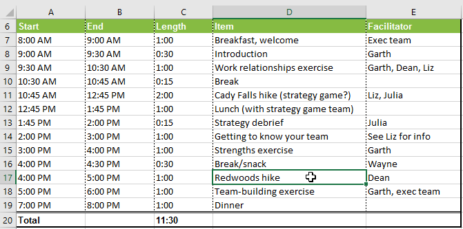
- From the Review tab, click the New Comment command.
- A comment box will appear. Type your comment, then click anywhere outside the box to close the comment.
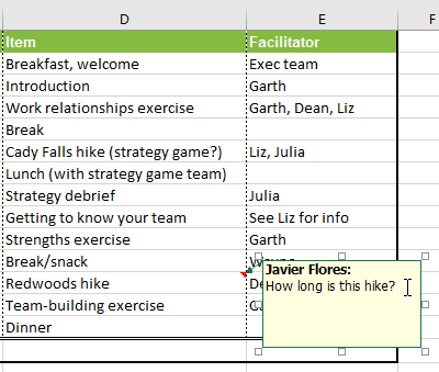
- The comment will be added to the cell, represented by the red triangle in the top-right corner.
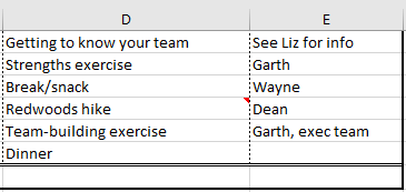
- Select the cell again to view the comment.
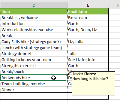
To edit a comment:
- Select the cell containing the comment you want to edit.
- From the Review tab, click the Edit Comment command.
- The comment box will appear. Edit the comment as desired, then click anywhere outside the box to close the comment.
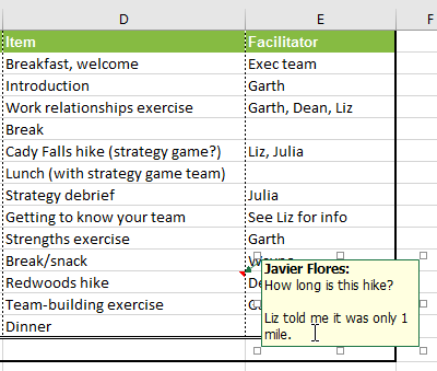
To show or hide comments:
- From the Review tab, click the Show All Comments command to view every comment in your worksheet at the same time.
- All comments in the worksheet will appear. Click the Show All Comments command again to hide them.
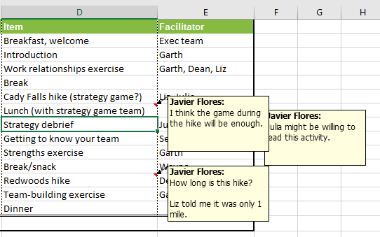
You can also choose to show and hide individual comments by selecting the desired cell and clicking the Show/Hide Comment command.
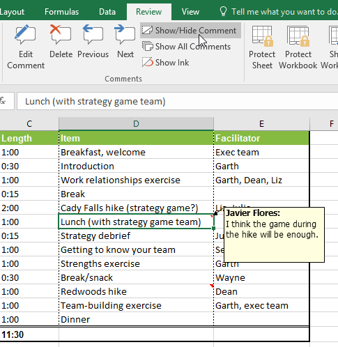
To delete a comment:
- Select the cell containing the comment you want to delete. In our example, we'll select cell E13.
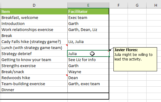
- From the Review tab, click the Delete command in the Comments group.
- The comment will be deleted.
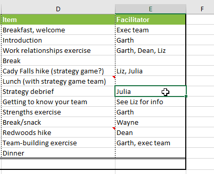
Challenge!
- Open our practice workbook.
- Turn on Track Changes.
- Replace the value in cell D14 with Rope Bridge Activity.
- Change cell E15 to say Julia.
- Save your workbook.
- List changes on a new sheet. After you do this, the worksheet should look like this:
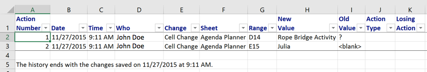
- Return to the Agenda Planner tab.
- Add a comment to cell E16 that says snacks will be provided by the exec team.
- When you're finished, your workbook should look like this:
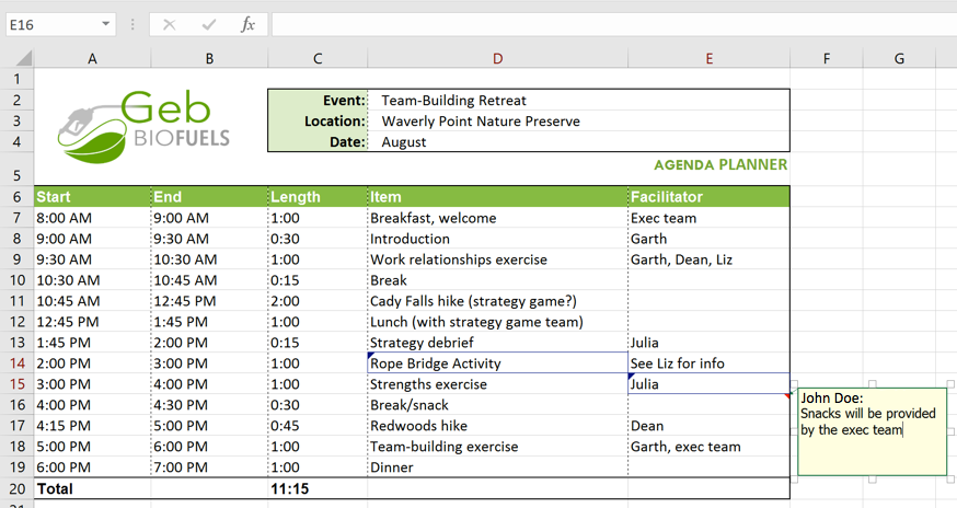
- Accept All Changes, then turn off Track Changes.
Lesson 26: Inspecting and Protecting Workbooks
Introduction
Before sharing a workbook, you'll want to make sure it doesn't include any spelling errors or information you want to keep private. Fortunately, Excel includes several tools to help finalize and protect your workbook, including Document Inspector and the Protect Workbook feature.
Optional: Download our practice workbook.
Watch the video below to learn more about inspecting and protecting workbooks.
Document Inspector
Whenever you create or edit a workbook, certain personal information may be added to the file automatically. You can use Document Inspector to remove this information before sharing a workbook with others.
Because some changes may be permanent, it's a good idea to save an additional copy of your workbook before using the Document Inspector to remove information.
To use Document Inspector:
- Click the File tab to access Backstage view.
- From the Info pane, click Check for Issues, then select Inspect Document from the drop-down menu.
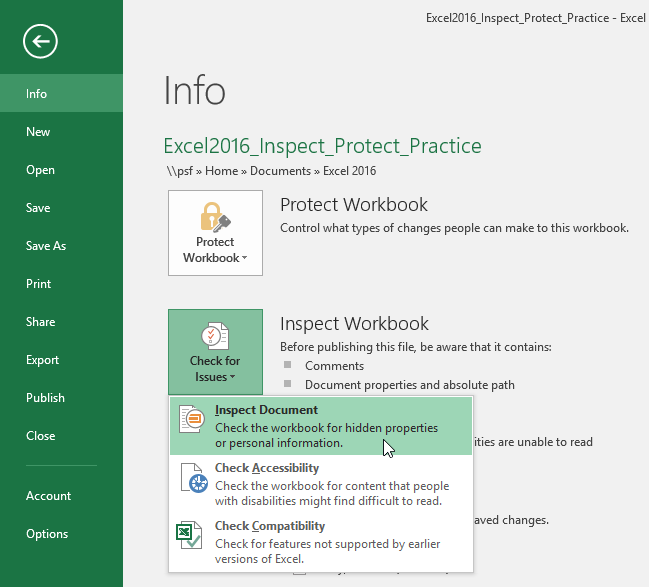
- You may be prompted to save your file before running Document Inspector.
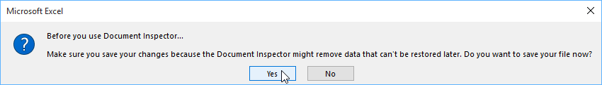
- Document Inspector will appear. Check or uncheck boxes, depending on the content you want to review, then click Inspect. In our example, we'll leave everything selected.
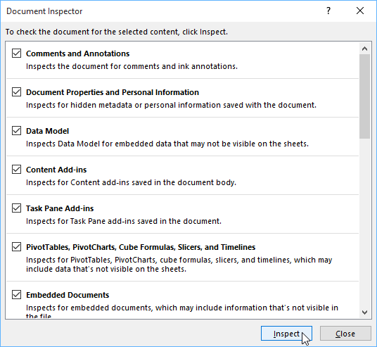
- The inspection results will appear. In our example, we can see that our workbook contains comments and some personal information, so we'll click Remove All on both items to remove this information from the workbook.
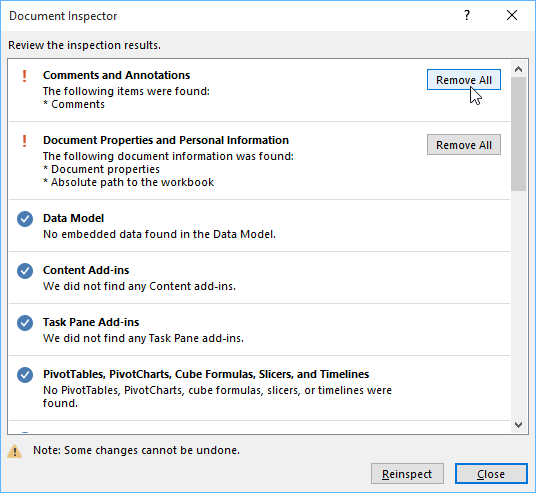
- When you're done, click Close.
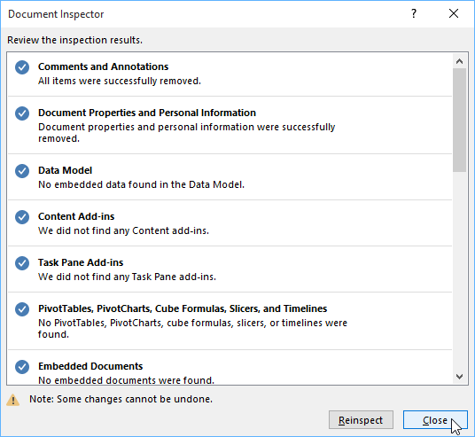
Protecting your workbook
By default, anyone with access to your workbook will be able to open, copy, and edit its content unless you protect it. There are many different ways to protect a workbook, depending on your needs.
To protect your workbook:
- Click the File tab to access Backstage view.
- From the Info pane, click the Protect Workbook command.
- In the drop-down menu, choose the option that best suits your needs. In our example, we'll select Mark as Final. Marking your workbook as final is a good way to discourage others from editing the workbook, while the other options give you even more control if needed.
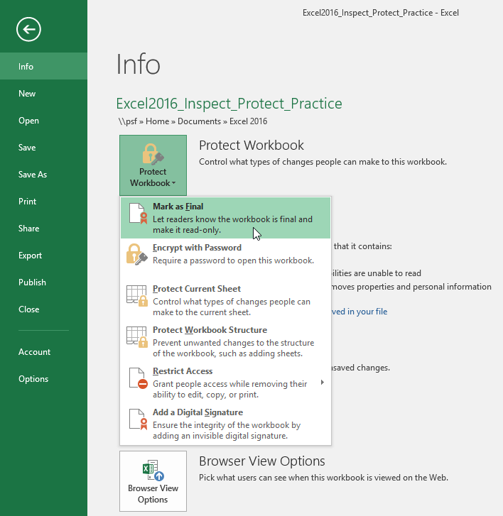
- A dialog box will appear, prompting you to save. Click OK.
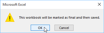
- Another dialog box will appear. Click OK.
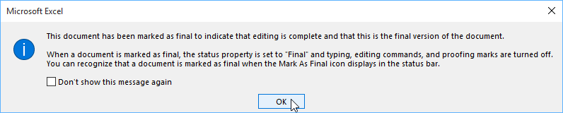
- The workbook will be marked as final.
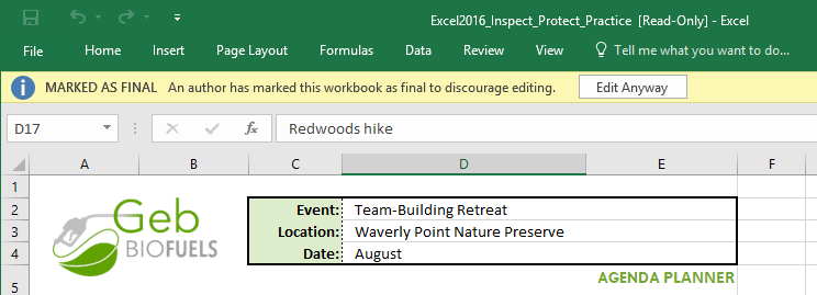
Marking a workbook as final will not prevent others from editing it. If you want to prevent people from editing it, you can use the Restrict Access option instead.
Challenge!
- Open our practice workbook.
- Use Document Inspector to check the workbook and remove anything it finds.
- Protect the workbook by Marking As Final.
- When you're finished, your workbook should look something like this:
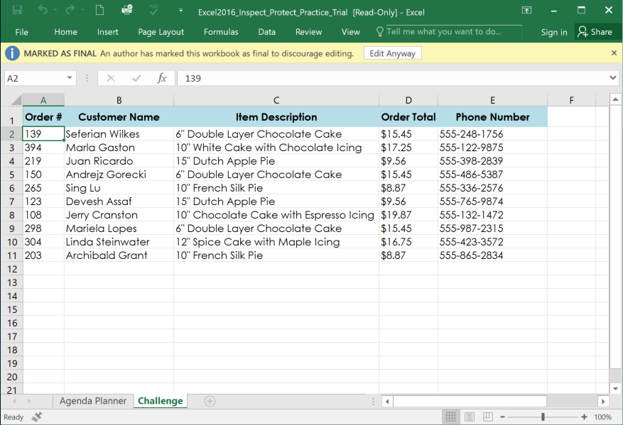
Lesson 27: Intro to PivotTables
Introduction
When you have a lot of data, it can sometimes be difficult to analyze all of the information in your worksheet. PivotTables can help make your worksheets more manageable by summarizing your data and allowing you to manipulate it in different ways.
Optional: Download our practice workbook.
Watch the video below to learn more about PivotTables.
Using PivotTables to answer questions
Consider the example below. Let's say we wanted to answer the question What is the amount sold by each salesperson? Answering it could be time consuming and difficult; each salesperson appears on multiple rows, and we would need to total all of their different orders individually. We could use the Subtotal command to help find the total for each salesperson, but we would still have a lot of data to work with.
Fortunately, a PivotTable can instantly calculate and summarize the data in a way that will make it much easier to read. When we're done, the PivotTable will look something like this:
Once you've created a PivotTable, you can use it to answer different questions by rearranging—or pivoting—the data. For example, let's say we wanted to answer What is the total amount sold in each month? We could modify our PivotTable to look like this:
To create a PivotTable:
- Select the table or cells (including column headers) you want to include in your PivotTable.
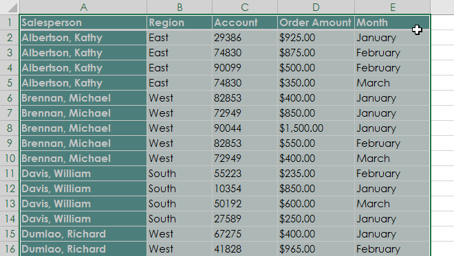
- From the Insert tab, click the PivotTable command.
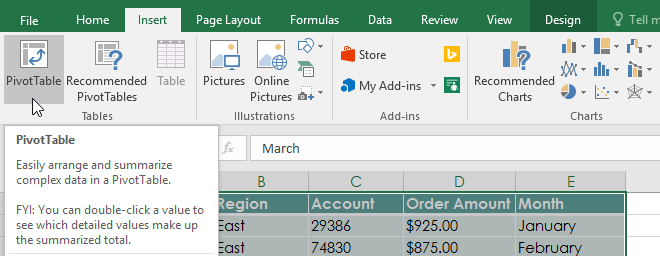
- The Create PivotTable dialog box will appear. Choose your settings, then click OK. In our example, we'll use Table1 as our source data and place the PivotTable on a new worksheet.
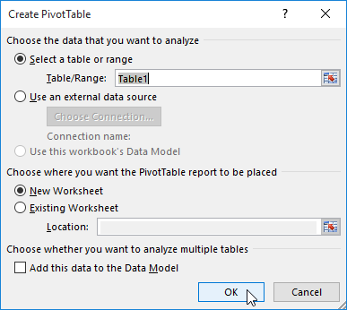
- A blank PivotTable and Field List will appear on a new worksheet.
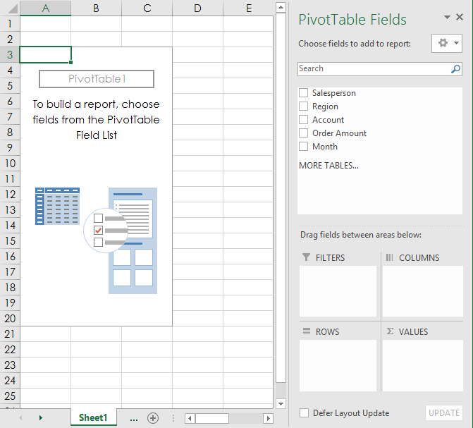
- Once you create a PivotTable, you'll need to decide which fields to add. Each field is simply a column header from the source data. In the PivotTable Field List, check the box for each field you want to add. In our example, we want to know the total amount sold by each salesperson, so we'll check the Salesperson and Order Amount fields.
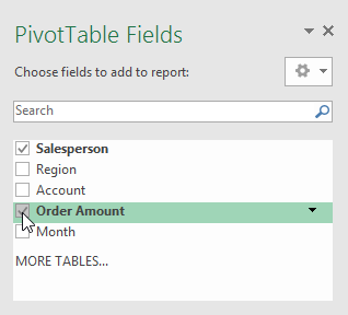
- The selected fields will be added to one of the four areas below. In our example, the Salesperson field has been added to the Rows area, while Order Amount has been added to Values. Alternatively, you can drag and drop fields directly into the desired area.
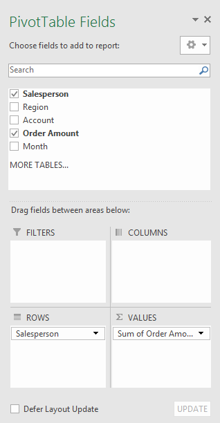
- The PivotTable will calculate and summarize the selected fields. In our example, the PivotTable shows the amount sold by each salesperson.
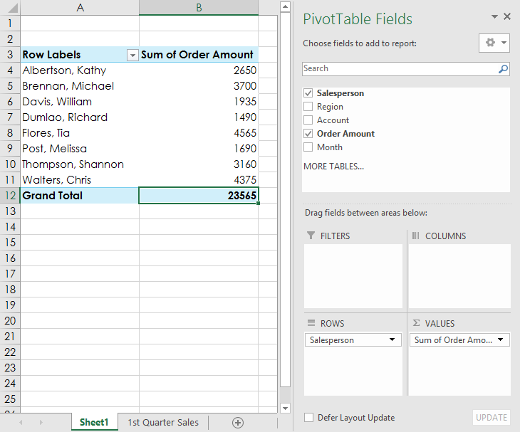
Just like with normal spreadsheets, you can sort the data in a PivotTable using the Sort & Filter command on the Home tab. You can also apply any type of number formatting you want. For example, you may want to change the number format to Currency. However, be aware that some types of formatting may disappear when you modify the PivotTable.
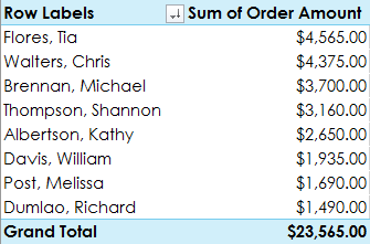
If you change any of the data in your source worksheet, the PivotTable will not update automatically. To manually update it, select the PivotTable and then go to Analyze Refresh.
Pivoting data
One of the best things about PivotTables is that they can quickly pivot—or reorganize—your data, allowing you to examine your worksheet in several ways. Pivoting data can help you answer different questions and even experiment with your data to discover new trends and patterns.
To add columns:
So far, our PivotTable has only shown one column of data at a time. In order to show multiple columns, you'll need to add a field to the Columns area.
- Drag a field from the Field List into the Columns area. In our example, we'll use the Month field.
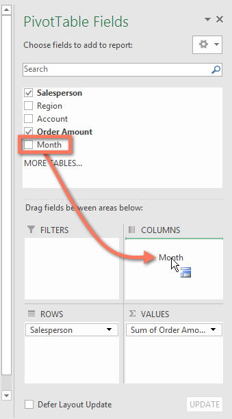
- The PivotTable will include multiple columns. In our example, there is now a column for each person's monthly sales, in addition to the grand total.
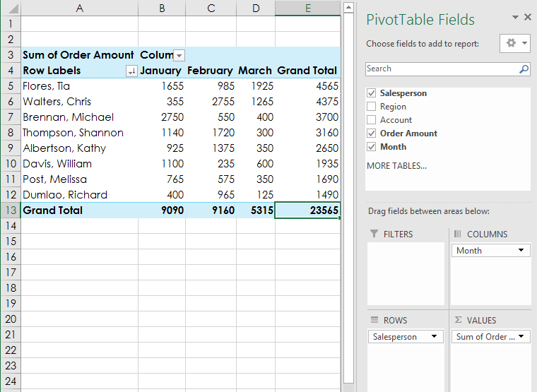
To change a row or column:
Changing a row or column can give you a completely different perspective on your data. All you have to do is remove the field in question, then replace it with another.
- Drag the field you want to remove out of its current area. You can also uncheck the appropriate box in the Field List. In this example, we've removed the Month and Salesperson fields.
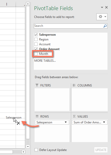
- Drag a new field into the desired area. In our example, we'll place the Region field under Rows.
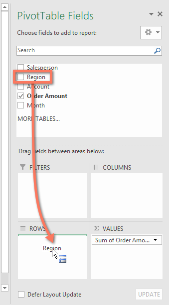
- The PivotTable will adjust—or pivot—to show the new data. In our example, it now shows the amount sold by each region.
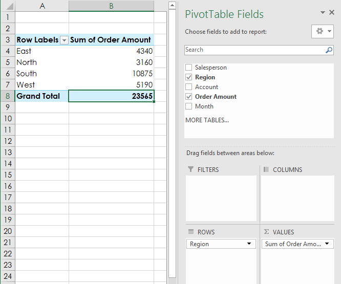
To learn more
Once you're comfortable with PivotTables, check out our Doing More with PivotTables lesson for even more ways to customize and manipulate them.
Challenge!
- Open our practice workbook.
- Create a PivotTable in a separate sheet.
- We want to answer the question What is the total amount sold in each region? To do this, select Region and Order Amount. When you're finished, your workbook should look like this:
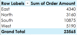
- In the Rows area, remove Region and replace it with Salesperson.
- Add Month to the Columns area.
- Change the number format of cells B5:E13 to Currency. Note: You might have to make columns C and D wider in order to see the values.
- When you're finished, your workbook should look like this:
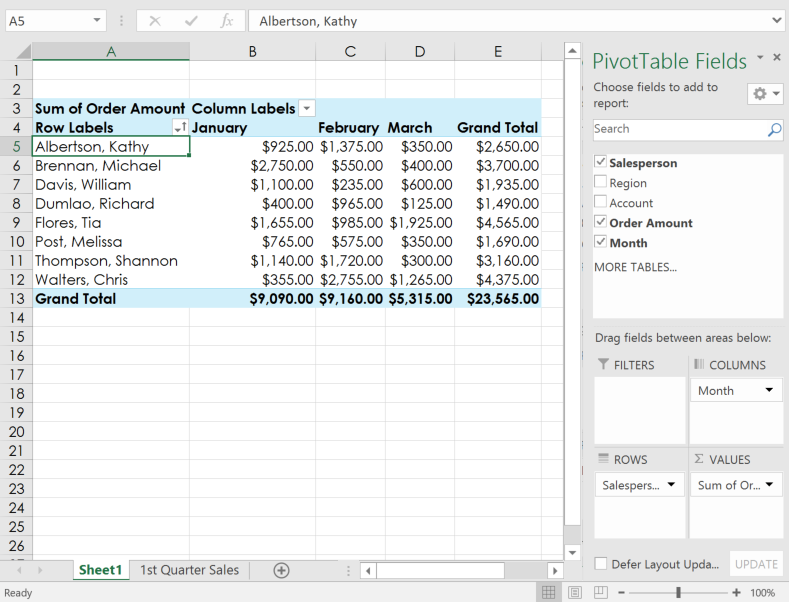
Lesson 28: Doing More with PivotTables
Introduction
As you learned in our previous lesson, Intro to PivotTables, PivotTables can be used to summarize and analyze almost any type of data. To help you manipulate your PivotTable—and gain even more insight into your data—Excel offers three additional tools: filters, slicers, and PivotCharts.
Optional: Download our practice workbook.
Watch the video below to learn more about enhancing PivotTables.
Filters
Sometimes you may want focus on a certain section of your data. Filters can be used to narrow down the data in your PivotTable, so you can view only the information you need.
To add a filter:
In the example below, we'll filter out certain salespeople to determine how their individual sales are impacting each region.
- Drag a field from the Field List to the Filters area. In this example, we'll use the Salesperson field.
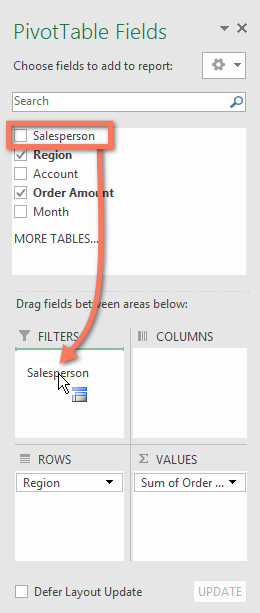
- The filter will appear above the PivotTable. Click the drop-down arrow, then check the box next to Select Multiple Items.
- Uncheck the box next to any item you don't want to include in the PivotTable. In our example, we'll uncheck the boxes for a few salespeople, then click OK.
- The PivotTable will adjust to reflect the changes.
Slicers
Slicers make filtering data in PivotTables even easier. Slicers are basically just filters but are easier and faster to use, allowing you to instantly pivot your data. If you frequently filter your PivotTables, you may want to consider using slicers instead of filters.
To add a slicer:
- Select any cell in the PivotTable.
- From the Analyze tab, click the Insert Slicer command.
- A dialog box will appear. Check the box next to the desired field. In our example, we'll select Salesperson, then click OK.
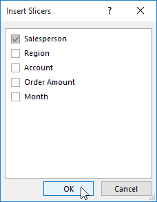
- The slicer will appear next to the PivotTable. Each selected item will be highlighted in blue. In the example below, the slicer contains all eight salespeople, but only five of them are currently selected.
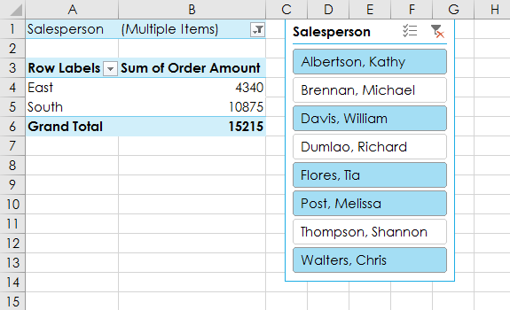
- Just like filters, only selected items are used in the PivotTable. When you select or deselect an item, the PivotTable will instantly reflect the change. Try selecting different items to see how they affect the PivotTable. Press and hold the Ctrl key on your keyboard to select multiple items at once.
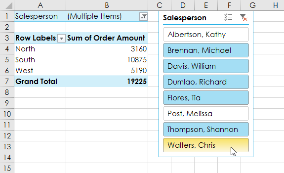
You can also click the Filter icon in the top-right corner of the slicer to select all items at once.
PivotCharts
PivotCharts are like regular charts, except they display data from a PivotTable. Just like regular charts, you'll be able to select a chart type, layout, and style that will best represent the data.
To create a PivotChart:
In the example below, our PivotTable is showing a portion of each region's sales figures. We'll use a PivotChart so we can see the information more clearly.
- Select any cell in your PivotTable.
- From the Insert tab, click the PivotChart command.
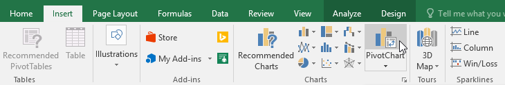
- The Insert Chart dialog box will appear. Select the desired chart type and layout, then click OK.
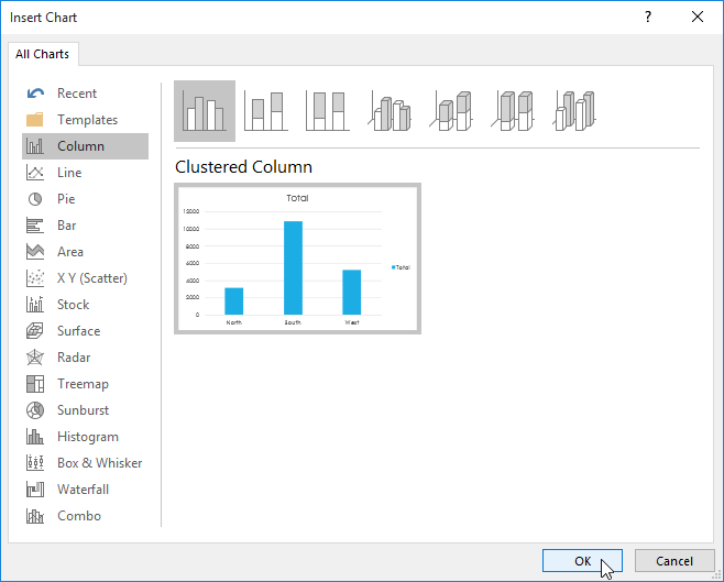
- The PivotChart will appear.
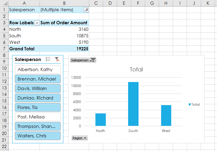
Try using filters or slicers to narrow down the data in your PivotChart. To view different subsets of information, change the columns or rows in your PivotTable. In the example below, we've changed the PivotTable to view the monthly sales for each salesperson.
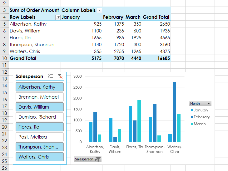
Challenge!
- Open our practice workbook.
- In the Rows area, remove Region and replace it with Salesperson.
- Insert a PivotChart, and choose the type Line with Markers.
- Insert a slicer for Regions.
- Use the slicer to only show the South and East regions.
- Change the PivotChart type to Stacked Column.
- In the PivotChart Fields pane to the right, add Month to the Legend (Series) area. Note: You can also click the PivotTable and then add Month to the Columns area; the result will be the same.
- When you're finished, your workbook should look something like this: